
The Lidar Radar Open Software Environment (LROSE) is an National Science Foundation (NSF) supported project to develop common software for the Lidar, Radar, and Profiler community based on collaborative, open source development. The core package is being jointly developed by Colorado State University (CSU) and the Earth Observing Laboratory at the NSF National Center for Atmospheric Research (NSF NCAR/EOL). The current LROSE release is called Colette (a versatile climbing rose).
More information on LROSE can be found on the LROSE wiki.
Notebook Summary
This notebook will cover the following:
- LROSE Overview
- LROSE on the Command Line
- LROSE Parameter Files
- Inspect the Data
- Format Conversion
- Simple Gridding
- Basic Data Display
LROSE Overview
LROSE encompasses six key toolsets that define a core lidar/radar workflow: Convert, Display, QC, Grid, Echo, and Winds. Colette focuses on high-quality, well-tested, well-maintained and well-documented key applications as ‘building blocks’, allowing users to assemble trusted, reproducible workflows to accomplish more complex scientific tasks.
Installation
LROSE is available for download through GitHub. Installation is supported for Linux (source, packages) and Mac OS (source, Homebrew). Conda-forge development is underway.
LROSE Tutorials
We’re developing a Science Gateway where LROSE tools are installed on NSF’s Jetstream2 supercomputer. The tutorials from that Gateway can also be found on GitHub.
https://
Issues?
For problems running LROSE or general questions, please reach out on the LROSE forum.
Please submit bugs on GitHub.
Listserv
We maintain a listserv to alert the LROSE community of new LROSE releases, workshops, and other general communication. Email traffic is generally minimal.
https://
Initialize python
import warnings

warnings.filterwarnings("ignore")

import os
import fsspec
import glob
import numpy as np
import matplotlib.pyplot as plt
import matplotlib.ticker as plticker
from matplotlib.lines import Line2D
import cartopy.crs as ccrs
import cartopy.io.shapereader as shpreader
import cartopy.geodesic as cgds
from cartopy.mpl.gridliner import LONGITUDE_FORMATTER, LATITUDE_FORMATTER
from cartopy import feature as cfeature
import xarray as xr
import pyart
# Set directory variable to call LROSE
os.environ["LROSE_DIR"] = "/usr/local/lrose/bin"
# Set the URL and path to access the data on the cloud
URL = "https://js2.jetstream-cloud.org:8001/"
path = f"pythia/radar/erad2024"
fs = fsspec.filesystem("s3", anon=True, client_kwargs=dict(endpoint_url=URL))
fs.glob(f"{path}/20240522_MeteoSwiss_ARPA_Lombardia/Data/Cband/*")
files = fs.glob(
f"{path}/20240522_MeteoSwiss_ARPA_Lombardia/Data/Cband/*.nc"
) #### FIX PATH
local_files = [
fsspec.open_local(
f"simplecache::{URL}{i}", s3={"anon": True}, filecache={"cache_storage": "."}
)
for i in files
]files[0]# create a directory
!mkdir -p ./raw
# LROSE prefers files to have .nc extension, so create a softlink with the actual filename
# We'll use the first file as an example!
os.system("ln -sf " + local_files[0] + " ./raw/" + files[0].split("/")[-1])!pwdLROSE on the Command Line
Each LROSE application has different command line options for running. To see all the available options, use the -h flag.
RadxPrint -h# view the command line options
!${LROSE_DIR}/RadxPrint -hLROSE Parameter Files
All LROSE applications have a detailed parameter file, which is read in at startup. The parameters allow the user to control the processing in the LROSE apps. To generate a default parameter file, you use the -print_params option for the app.
For example, for RadxConvert you would use:
RadxConvert -print_params > RadxConvert.nexradand then edit RadxConvert.nexrad appropriately.
At runtime you would use:
RadxConvert -params RadxConvert.nexrad ... etc ...# view the default parameters
!${LROSE_DIR}/RadxPrint -print_params# save the default parameters to a file
!${LROSE_DIR}/RadxPrint -print_params > ./RadxPrint_params
# if you have an existing parameter file and want to update it (e.g., a new LROSE version is released),
# you could run a command similar to the following, just update the parameter file names
# !${LROSE_DIR}/RadxPrint -f ./path/to/RadxPrint_params -print_params > ./RadxPrint_params_new# View the param file
!cat ./RadxPrint_paramsInspect the Data
RadxPrint can print out file metadata, information about the variables, and other data. It’s an alternative to ncdump, depending on the information you want.
# Print the metadata for the file we linked to earlier (-f flag links to files)
!${LROSE_DIR}/RadxPrint -f ./raw/*.nc
# Examine ray-specific metadata
!${LROSE_DIR}/RadxPrint -summary -f ./raw/*.nc | tail -200Format Conversion
RadxConvert can convert many different file types into CfRadial files, which are used by most LROSE applications. You can specify specific parameters in a parameter file, but most of the time, RadxConvert works with a simple command.
# Convert file (already cfradial, but you get the idea)
# this will create a new subdirectory called convert along with a subdirectory YYYYMMDD that contains the file
!${LROSE_DIR}/RadxConvert -f ./raw/*.nc -outdir ./convert
Simple Gridding
Another commonly-used applicated is Radx2Grid, which regrids data onto a Cartesian grid. Usually, a user will want to specify parameters in a parameter file, but for the sake of time, we’ll just use the defaults to show how the application works.
!${LROSE_DIR}/Radx2Grid -f ./convert/*/*.nc -outdir ./griddedBasic Data Display
With these files, we can plot the output to look at the data. Here, we’ll use Py-ART to plot the data in the CfRadial file and xarray/matplotlib to plot the gridded data.
Plotting CfRadial data with Py-ART
# Read CfRadial file into radar object
filePath = os.path.join(
    "./", "convert/20240522/cfrad.20240522_125501.000_to_20240522_125944.950_L_SUR.nc"
)
radar = pyart.io.read_cfradial(filePath)
radar.info("compact")
display = pyart.graph.RadarDisplay(radar)
fig = plt.figure(1, (10, 10))
# DBZ
axDbz = fig.add_subplot(221)
display.plot_ppi(
"reflectivity",
0,
vmin=-32,
vmax=64.0,
axislabels=("x(km)", "y(km)"),
colorbar_label="DBZ",
)
display.plot_range_rings([50, 100, 150, 200])
display.plot_cross_hair(200.0)
# velocity
axKdp = fig.add_subplot(222)
display.plot_ppi(
"velocity",
0,
vmin=-15,
vmax=15,
axislabels=("x(km)", "y(km)"),
colorbar_label="velocity (m/s)",
)
display.plot_range_rings([50, 100, 150, 200])
display.plot_cross_hair(200.0)
# spectrum width
axHybrid = fig.add_subplot(223)
display.plot_ppi(
"spectrum_width", 0, axislabels=("x(km)", "y(km)"), colorbar_label="sw (m/s)"
)
display.plot_range_rings([50, 100, 150, 200])
display.plot_cross_hair(200.0)
# NCAR PID (computed)
axPID = fig.add_subplot(224)
display.plot_ppi(
"differential_reflectivity",
0,
axislabels=("x(km)", "y(km)"),
colorbar_label="ZDR (dB)",
)
display.plot_range_rings([50, 100, 150, 200])
display.plot_cross_hair(200.0)
fig.tight_layout()
plt.show()Plotting Gridded Data with xarray and matplotlib
# Read in example radar mosaic for a single time

filePathGridded = os.path.join("./", "gridded/20240522/ncf_20240522_125944.nc")
dsGridded = xr.open_dataset(filePathGridded)
print("Radar mosaic file path: ", filePathGridded)
print("Radar mosaic data set: ", dsGridded)

# Compute time

start_time = dsGridded["start_time"]
startTimeStr = start_time.dt.strftime("%Y/%m/%d-%H:%M:%S UTC")[0].values
print("Start time: ", startTimeStr)
minLonMosaic = 7
maxLonMosaic = 11
minLatMosaic = 44.5
maxLatMosaic = 47
# Create map for plotting lat/lon grids
def new_map(fig):
## Create projection centered on data
proj = ccrs.PlateCarree()
## New axes with the specified projection:
ax = fig.add_subplot(1, 1, 1, projection=proj)
## Set extent the same as radar mosaic
# ax.set_extent([minLonMosaic, maxLonMosaic, minLatMosaic, maxLatMosaic])
## Add grid lines & labels:
gl = ax.gridlines(
crs=ccrs.PlateCarree(),
draw_labels=True,
linewidth=1,
color="lightgray",
alpha=0.5,
linestyle="--",
)
gl.top_labels = False
gl.left_labels = True
gl.right_labels = False
gl.xlines = True
gl.ylines = True
gl.xformatter = LONGITUDE_FORMATTER
gl.yformatter = LATITUDE_FORMATTER
gl.xlabel_style = {"size": 8, "weight": "bold"}
gl.ylabel_style = {"size": 8, "weight": "bold"}
return ax# Plot column-max reflectivity
figDbzComp = plt.figure(figsize=(8, 8), dpi=150)
axDbzComp = new_map(figDbzComp)
plt.imshow(
dsGridded["reflectivity"].sel(z0=4.5).isel(time=0),
cmap="pyart_Carbone42",
interpolation="bilinear",
origin="lower",
extent=([minLonMosaic, maxLonMosaic, minLatMosaic, maxLatMosaic]),
)
axDbzComp.add_feature(cfeature.BORDERS, linewidth=0.5, edgecolor="black")
axDbzComp.add_feature(cfeature.STATES, linewidth=0.3, edgecolor="brown")
# axDbzComp.coastlines('10m', 'darkgray', linewidth=1, zorder=0)
plt.colorbar(label="DBZ", orientation="vertical", shrink=0.5)
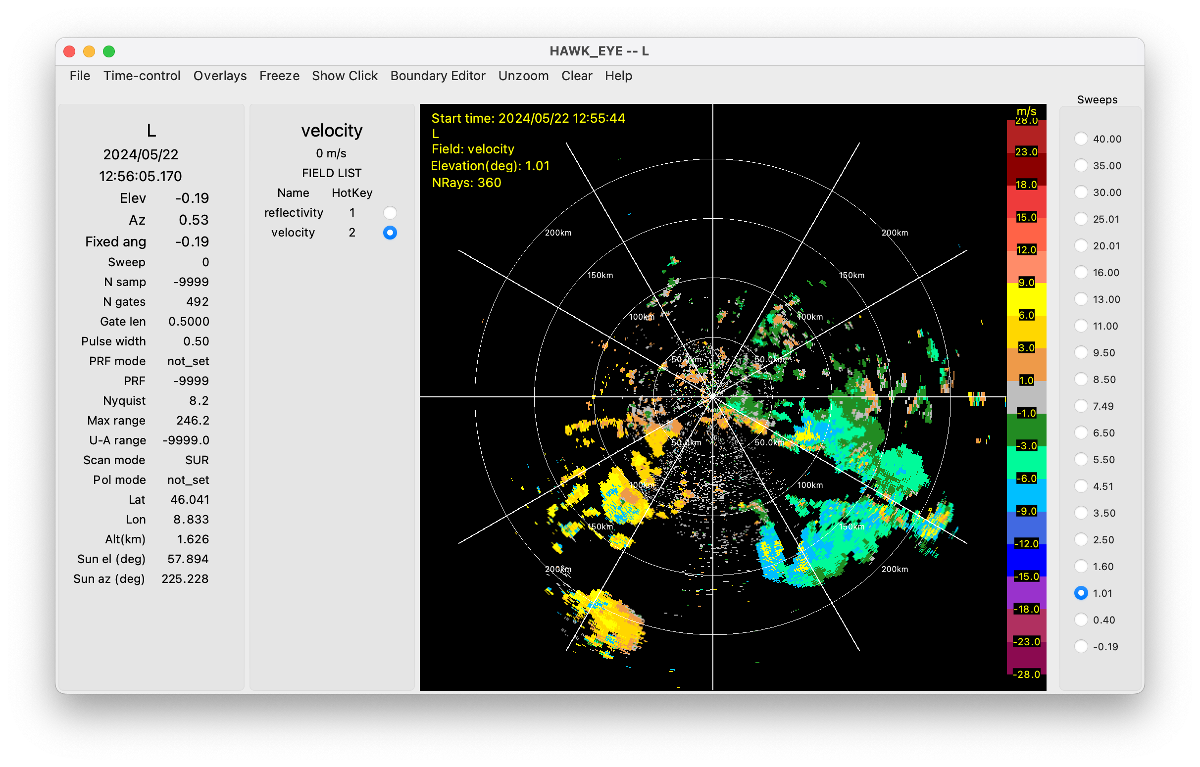
plt.title("Radar DBZ: " + startTimeStr)Hawkeye
We also have an application called HawkEye that displays CfRadial radar data. It’s useful for switching between different sweeps and files.
Afternoon preview
Want to learn how to run multi-Doppler analysis using FRACTL and SAMURAI? Join us in the afternoon!
Additional resources
More tutorials can be found on our Gateway GitHub repo:
https://
The LROSE wiki can be found here:
http://
The LROSE forum can be found here:
http://