Using HighIQ
Input and Output
HighIQ uses NetCDF files as its inputs. Currently, the I/O module supports NetCDF files that conform to Atmospheric Radiation Measurement standards. Therefore, in order to place data into a format supported by HighIQ, a data ingest must be able to place the data in xarray datasets that contain 3D variables that have dimensions of (time, nsamples, complex). These dimensions are defined as:
time = the number of samples in time
nsamples = the number of given samples for a ray
complex = index 0 is real component of ACF, 1 is imaginary component.
The complex dimension will always be of length 2. This array will store the ACF for the radar or lidar signal. In addition, HighIQ also expects a background ACF for determining the noise floor of the instrument. This background ACF array will have the same dimensions as the ACF array.
After the acf array has been created (or loaded using xarray.open_dataset), the
next step is to create the Doppler spectra using highiq.calc.get_psd():
$ my_ds = highiq.calc.get_psd(my_ds)
Read the documentation on highiq.calc.get_psd() in order to learn how to
customize parameters such as the size of the range gate, sampling frequency, and
number of points to include in the FFT. This function will add Doppler spectra
variables ‘power_spectra_density’ which contains the power spectral density in
\(dB\ m\ s^{-1}\) and ‘power_spectra_density_normed’ which is normalized
such that the integral under the curve is 100%. The power spectra density are defined
at nfft points between the negative and positive Nyquist velocities of the
radar or lidar.
However, while nfft can be the optimal number of points to include in the FFT, for a robust calculation of moments, interpolation of the Doppler spectra are required. Therefore, In addition, HighIQ will interpolate the Doppler spectra generated over the original nfft point space in order to provide smoother Doppler spectra more suitable for the calculation of the moments of the spectra.
After these Doppler spectra are created, the calculation of the lidar moments is as easy as:
$ my_moments = highiq.calc.get_lidar_moments(my_ds)
Optimizing processing
For both the processing of the Doppler spectra and moments, HighIQ will only store
a portion of the dataset in the GPU’s memory due to limitations. However, if you
have a high amount of GPU memory, you may be able to optimize the processing
by increasing the block_size_ratio keyword of both highiq.calc.get_lidar_moments() and
highiq.calc.get_psd().
Plotting Spectra
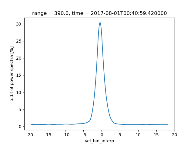
Since the output arrays are xarray Datasets, the standard xarray plotting routines can be used to make visualizations. For example, in order to plot the Doppler spectra from the example file, we simply do:
$ # Load the data. This uses a module in the Atmospheric Community
$ # Toolkit to ensure that the input acf data are always
$ # entered into a 3D array of (time, nsamples, complex)
$
$ my_ds = highiq.io.load_arm_netcdf(highiq.testing.TEST_FILE)
$ my_ds_processed = highiq.calc.get_psd(my_ds)
$
$ # For plotting the spectra, simply use xarray's built in functionality
$ #
$ my_ds_processed.power_spectra_normed_interp.sel(range=400, method='nearest').plot()

The above example chooses the range gate that is 400 m away from the radar and will plot
the Doppler spectra at that point. In this example, we are using the single test data point
file that is contained within HighIQ’s test file. For files with multiple time periods,
selecting by time period is as easy as specifying a time keyword to the sel function in last line in
the above example. The format of this time is a datetime, so selecting 2018-08-01 00:40:00 UTC would mean
adding a time=datetime(2018, 8, 1, 0, 40, 0) to the list of keywords.
Plotting 2D time series
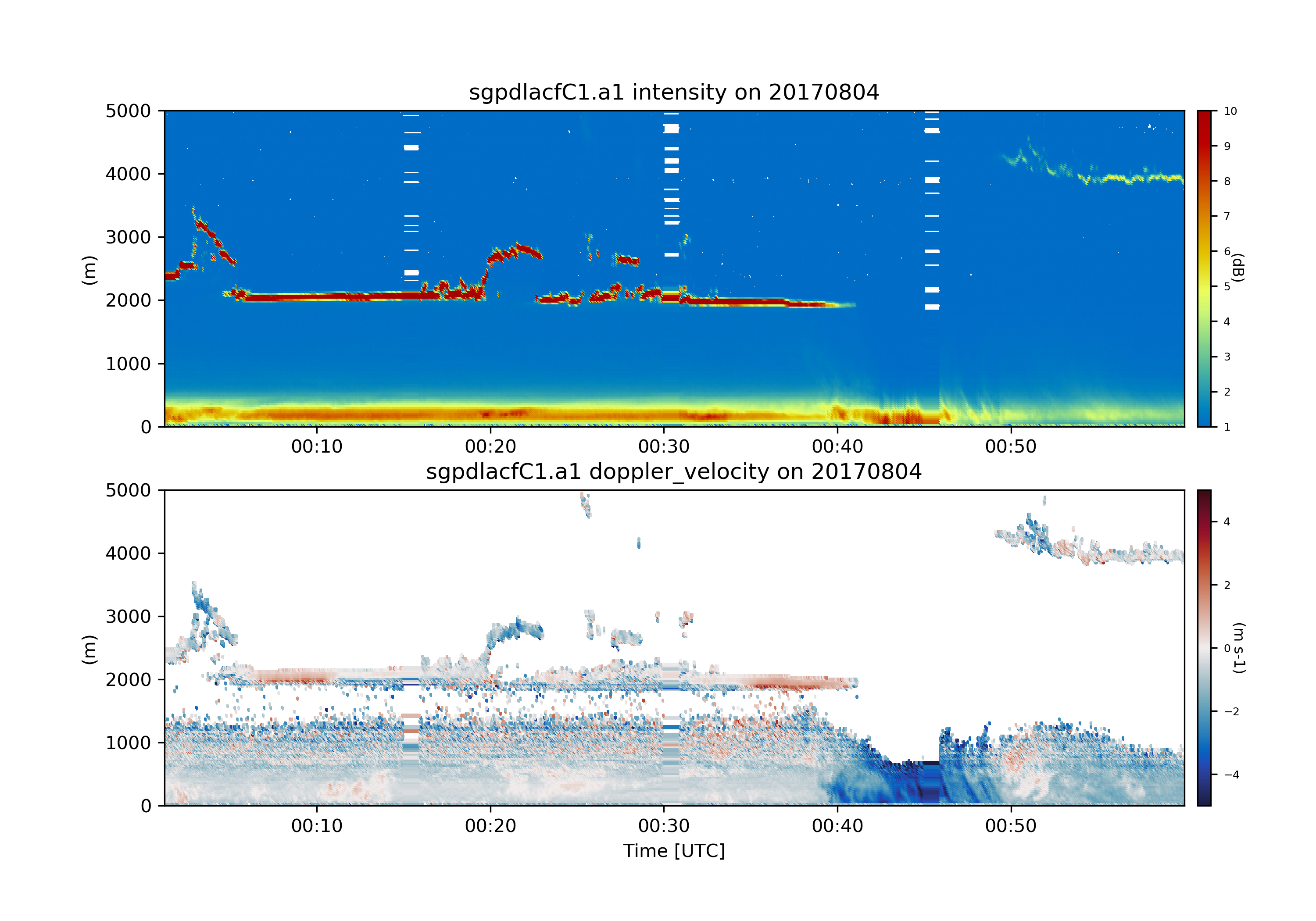
2D Visualization of spectra is easily done using the Atmospheric Community Toolkit (ACT). One is encouraged to read the documentation and examples from ACT in order to learn how to create custom visualizations. For the majority of vertically-pointing observations, ACT’s TimeSeriesDisplay object provides the functionality needed to create quicklook plots of the retrieved lidar moments. For example, in order to plot the radar moments from the example file, simply do:
$ import highiq
$ import act
$ my_ds = highiq.io.load_arm_netcdf('sgpdlacfC1.a1.20170804.000113.nc.v0')
$ my_ds = highiq.calc.get_psd(my_ds)
$ my_ds = highiq.calc.get_lidar_moments(my_ds)
$ # Make a stricter mask for Doppler velocity to favor excluding more noise
$ my_ds['doppler_velocity'] = my_ds['doppler_velocity'].where(my_ds.intensity > 1.2)

$ # With ACT, we set up a TimeSeriesDisplay object with two sub plots
$ my_display = act.plotting.TimeSeriesDisplay(my_ds, figsize=(10,7), subplot_shape=(2,))

$ # The plot function takes in the same kwargs as matplotlib's plotting routines
$ my_display.plot('intensity', subplot_index=(0,), cmap='act_HomeyerRainbow', vmin=1, vmax=10)
$ my_display.plot('doppler_velocity', subplot_index=(1,), cmap='act_balance', vmin=-5, vmax=5)
$ my_display.set_yrng([0, 5000], subplot_index=(0,))
$ my_display.set_yrng([0, 5000], subplot_index=(1,))
$ my_display.fig.savefig('spectra_difference.png', dpi=300)

This code will make two subplots that look like the image above.