ARCO Data Access
Canadian data was converted into Analysis-Ready Cloud-Optimized and can be accessed as follows
import xarray as xr
import icechunk
Configure S3 storage for icechunk. In this case we will analyze Ontario Derecho event. However, you can change it uncommenting the other prefix lines
storage = icechunk.s3_storage(
    bucket='pythia',
    # prefix='radar/ams2025/CASSM.zarr', # Calgary Hail Storm
    prefix='radar/ams2025/CASET.zarr', # CASET Ontario Derecho
    # prefix='radar/ams2025/CASKR.zarr', # CASKR Ontario Derecho
    endpoint_url='https://js2.jetstream-cloud.org:8001',
    anonymous=True,
    region='us-east-1',
    force_path_style=True
)
Creating S3 bucket connection and immutable session
repo = icechunk.Repository.open(storage=storage)
session = repo.readonly_session("main")
Opening the Radar datatree using xarray
dtree = xr.open_datatree(
    session.store,
    engine="zarr",
    consolidated=False,
    chunks={}
)dtreeLoading...
We have created a python script with additional functions to keep the notebook simple. If you want to check it out click here
import demo_functions as dmfwe can call the rain_depth function which will help us to compute QPE using Marshall and Gunn relationship
%%time
qpe = dmf.rain_depth(dtree["sweep_16/DBZH"])
Actual QPE integration period: 0 days, 3 hours, 54 minutes
Time span: 2022-05-21T14:54:03 to 2022-05-21T18:48:03 UTC
CPU times: user 6.55 ms, sys: 0 ns, total: 6.55 ms
Wall time: 6.53 ms
qpeLoading...
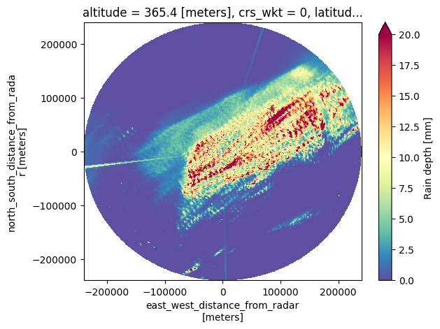
qpe_sum = qpe.sum("vcp_time")Finally, we can create a ~4 hour QPE plot as follows:
qpe_sum.plot(
    x="x",
    y="y",
    vmin=0,
    vmax=20,
    robust=True,
    cmap="Spectral_r",
    cbar_kwargs={"label": "Rain depth [mm]"},
)