ARCO Data Access
Canadian data was converted into Analysis-Ready Cloud-Optimized and can be accessed as follows
import xarray as xr
import icechunk
Configure S3 storage for icechunk. In this case we will analyze Calgary Hail Storm event. However, you can change it to Ontario Derecho by uncommenting the other prefix lines
storage = icechunk.s3_storage(
    bucket='pythia',
    prefix='radar/ams2025/CASSM.zarr', # Calgary Hail Storm
    # prefix='radar/ams2025/CASET.zarr', # CASET Ontario Derecho
    # prefix='radar/ams2025/CASKR.zarr', # CASKR Ontario Derecho

    endpoint_url='https://js2.jetstream-cloud.org:8001',
    anonymous=True,
    region='us-east-1',
    force_path_style=True
)
Creating S3 bucket connection and immutable session
repo = icechunk.Repository.open(storage=storage)
session = repo.readonly_session("main")
Opening the Radar datatree using xarray
dtree = xr.open_datatree(
    session.store,
    engine="zarr",
    consolidated=False,
    chunks={}
)dtreeLoading...
We have created a python script with additional functions to keep the notebook simple. If you want to check it out click here
import demo_functions as dmfwe can call the compute_qvp function which will help us to compute QVP for each vpol
%%time
ref_qvp = dmf.compute_qvp(dtree["sweep_1"], var="DBZH")
zdr_qvp = dmf.compute_qvp(dtree["sweep_1"], var="ZDR")
rhohv_qvp = dmf.compute_qvp(dtree["sweep_1"], var="RHOHV")
phidp_qvp = dmf.compute_qvp(dtree["sweep_1"], var="PHIDP")
CPU times: user 354 ms, sys: 30.6 ms, total: 385 ms
Wall time: 403 ms
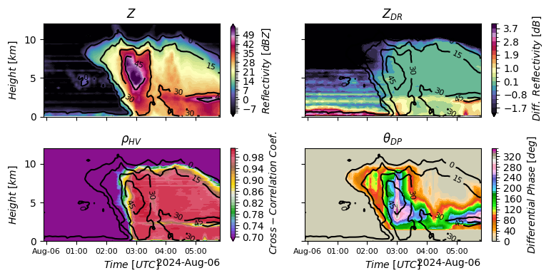
Finally, we can plot it using ryzhkov_figure function
%%time
dmf.ryzhkov_figure(ref_qvp, zdr_qvp, rhohv_qvp, phidp_qvp)
CPU times: user 2.03 s, sys: 130 ms, total: 2.16 s
Wall time: 3.56 s