COURSE: Open Radar - Open Source Software Tools for Radar Data Processing
ERAD - Rome, 9-13 September 2024
This notebook contains some high-level literature background for the multi-doppler analysis exercise at ERAD 2024.
Data acknowledgment: The data for the case used in the exercise is provided by the Meteorological Service of Catalonia.
Multi Doppler analysis
Multi-Doppler analysis consists on obtaining 3D wind fields using the radial observed velocity from two or more independent (non-collinearly located) Doppler radars. Techniques using Cylindrical and Cartesian coordinates systems are explained in Armijo 1969, Ray and Wagner 1976, and Ray and Sangren 1983, for instance. The mean radial velocity from every single radar is related to the rectangular components of the mean velocity (,, and ) through the azimuth (ϕ), and elevation (ε) angles (Fig.1).
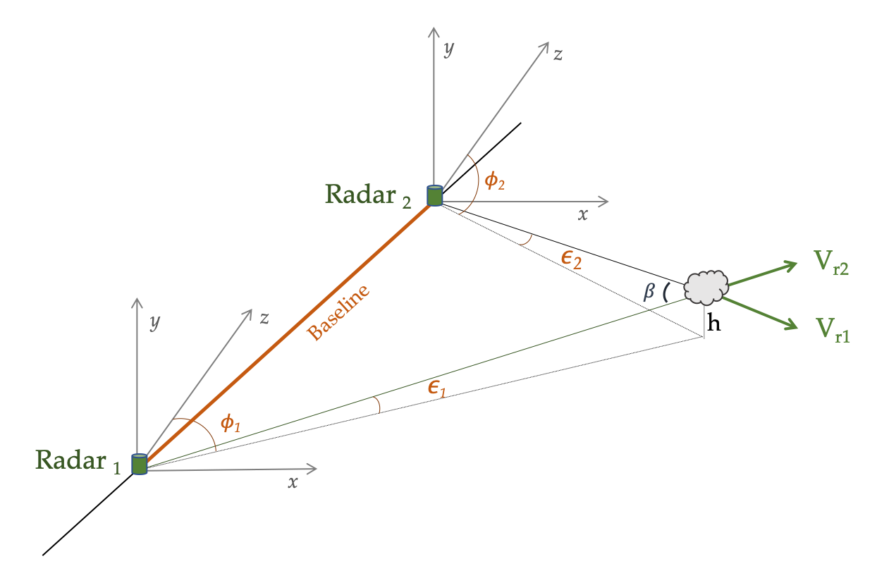
Fig 1: Dual-Doppler Cartesian geometry from two radars. Adapted from Rauber and Nesbitt (2018).
It is possible to obtain a unique solution for the horizontal and vertical velocities at a given point by combining the radial velocities in a closed equation system (more than two radars), or by applying boundary conditions on the vertical velocity and the terminal velocity of the hydrometeors (), and integrating the mass continuity equation (Miller and Strauch, 1974):
Dual Doppler coverage (2 radars)
We want our storm to be placed in the “optimal area” region, for which we need to know what is our Dual Doppler coverage and the optimal spatial resolution to resolve storm-related winds.
These are some things to consider:
The variance on the horizontal wind field is represented by the standard deviation of the local and components of the wind: and .
The variance of the radial velocity from each radar (spectral width) is represented by and .
Both variances represent the beam-crossing angle between the two radars (β), and consequently the “dual-Doppler lobes”:
Literature demonstrates that $\beta$=30º is one of the most suitable ones (e.g. Davies-Jones, 1979; Lhermitt and Miller, 1970; Friedrich and Hagen, 2004). This keeps the horizontal wind error below 3 m/s ($\sigma^{2}_u$ and $\sigma^{2}_v$) in convective situations*. The dual lobes centers are located perpendicular to the bisection of the baseline ($b$). The baseline is the distance separating the two radars (Fig. 2). The dual-lobes area is defined by: $$ A(\beta) = 2 (\frac{b}{2}\csc \beta )^{2} (\pi -2\beta +\sin 2\beta ) $$
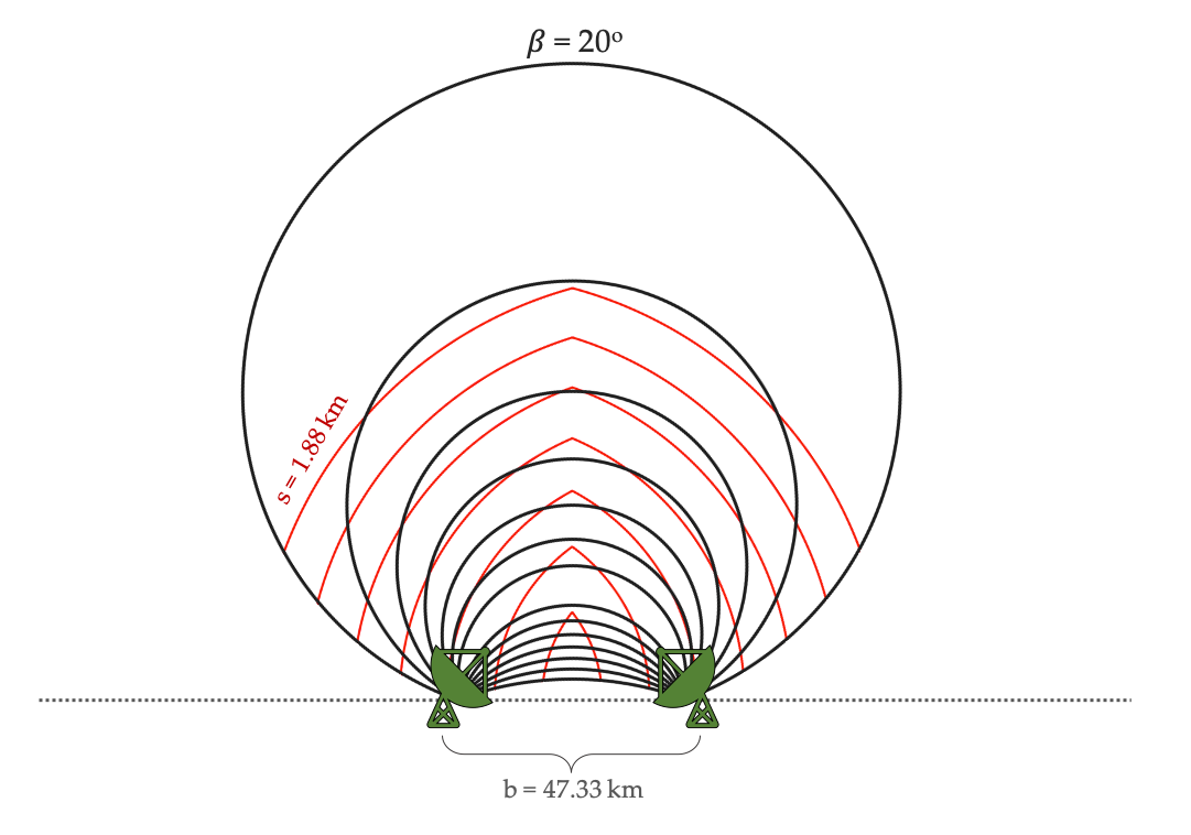
Fig 2: Dual-Doppler configuration with beam crossing angle ($\beta$), in black, and constant spatial resolution (s) for a beamwidht of 1.2° and a baseline b = 47.33 km. Adapted from (Davies-Jones, 1979)
Finally, it is also important to consider the spatial resolution .
The paired radars must be able to resolve horizontal scales below 3-6 km. This compromises the beam-crossing angle β and the baseline . If is too big, the data will degrade at the edges of the dual lobes due to the beam spread and elevation.
We will consider that the spatial resolution is proportional to the range , and approximately to the beam height:
where Δ is half of the beam width and 180º is expressed in degrees (Davies-Jones, 1979).
The area representing the region where points are at a distance , with a spatial resolution for 0º beam height is described in the following equation:
Case of analysis: Tornado in Catalonia - Jan 7, 2018
Dual Doppler coverage in Catalonia
The XRAD (Xarxa de RADars) is the radar network of the Meteorological Service of Catalonia (NE of Spain). The network is formed by four C-band single-Doppler radars, covering an area of ~ 32,114 km2 with complex terrain.
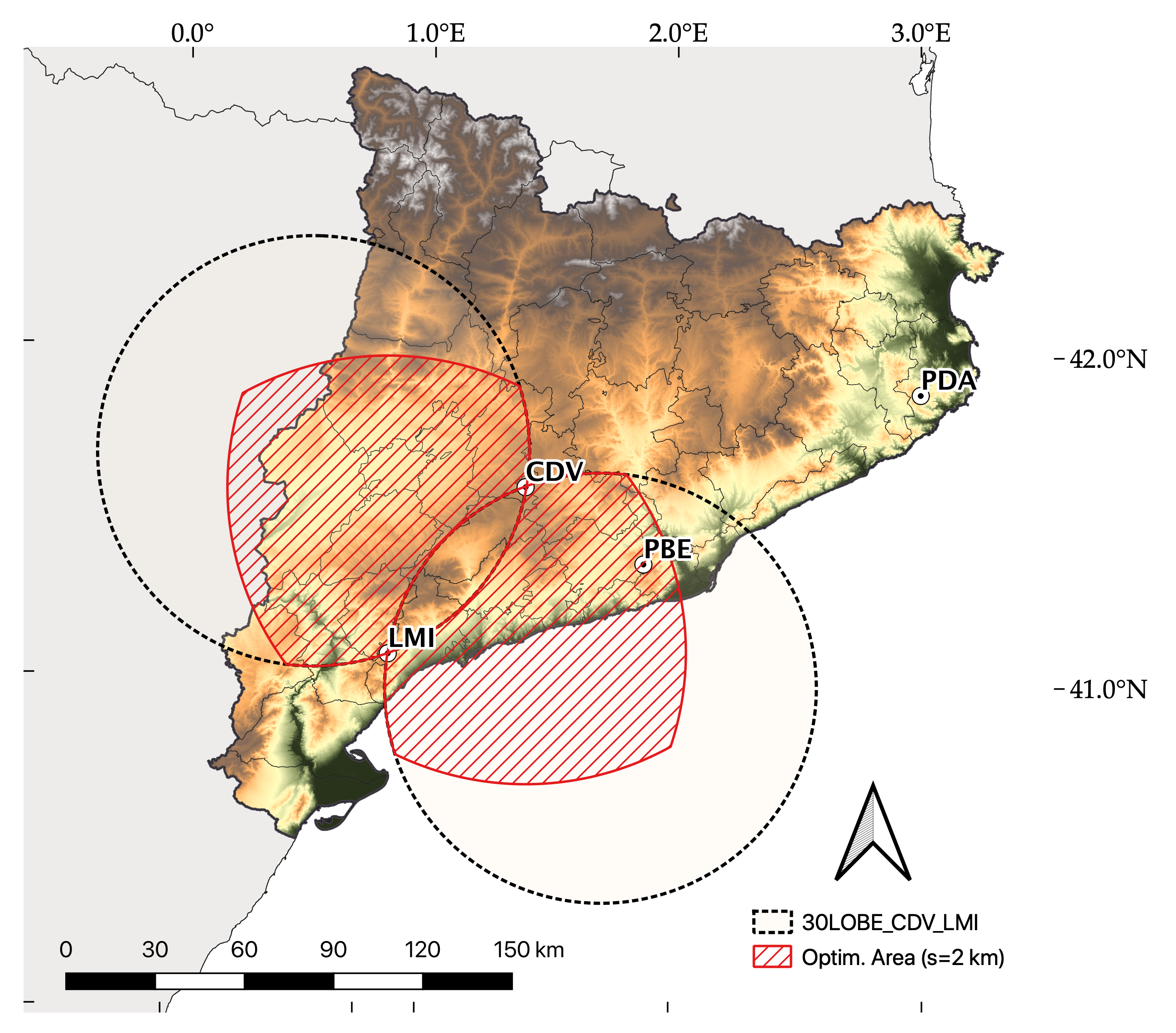
Del Moral Méndez 2020, and del Moral Méndez et al., 2020 explore the possible dual-Doppler coverage for the operational XRAD network and establish that with a maximum resolution of 2 km at the farthest point, and with 320deg dual-lobes, CDV-PBE and CDV-LMI are the two most suitable pairs of radars for dual-Doppler analysis.
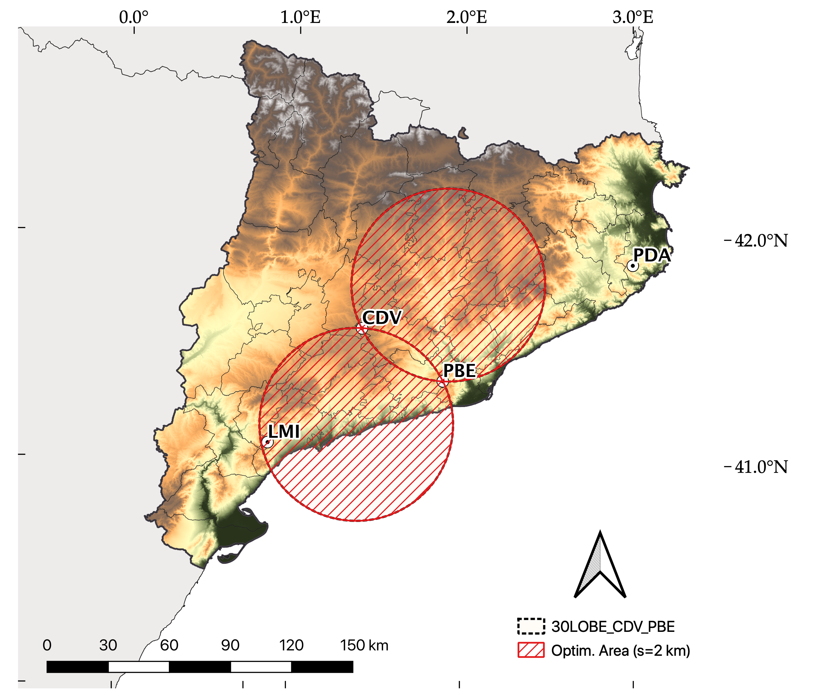
The two radars selected to analyse the tornado case are CDV-PBE, and the coverage is represeted in Fig. 3 (right). Notice that the “optimal area” is the intersection of the desired dual-lobe and the optimal resolution area. In this case, these two are the same. For this case and radar configuration, the baseline is 47.33 km, the farthest point is located at 94.66 km with a minimum resolution of 1.98 km. The lobes cover a total area of 13.303 km3 and with only 0.61% of topography blockage (del Moral et al. 2020)
Dual Doppler
Dual Doppler
Fig 3: Dual-Doppler coverage for the CDV-PBE and CDV-LMI pairs of radars (in red). The 30° dual-lobe is shown in dotted black circles.
Tornado track
The severe weather event on 6-7 January 2018 occurred outside the convective season in the northwestern Mediterranean. Several rain bands with a predominant southeasterly flow affected the area. Within those bands, embedded convective cells produced severe weather, causing two significant tornadoes, both rated EF2. The tornado in the central region of Catalonia was the result of a nocturnal supercell propagating NW and channeling through a narrow valley, and achieving speeds up tp 180 km/h with a 500 m diameter.
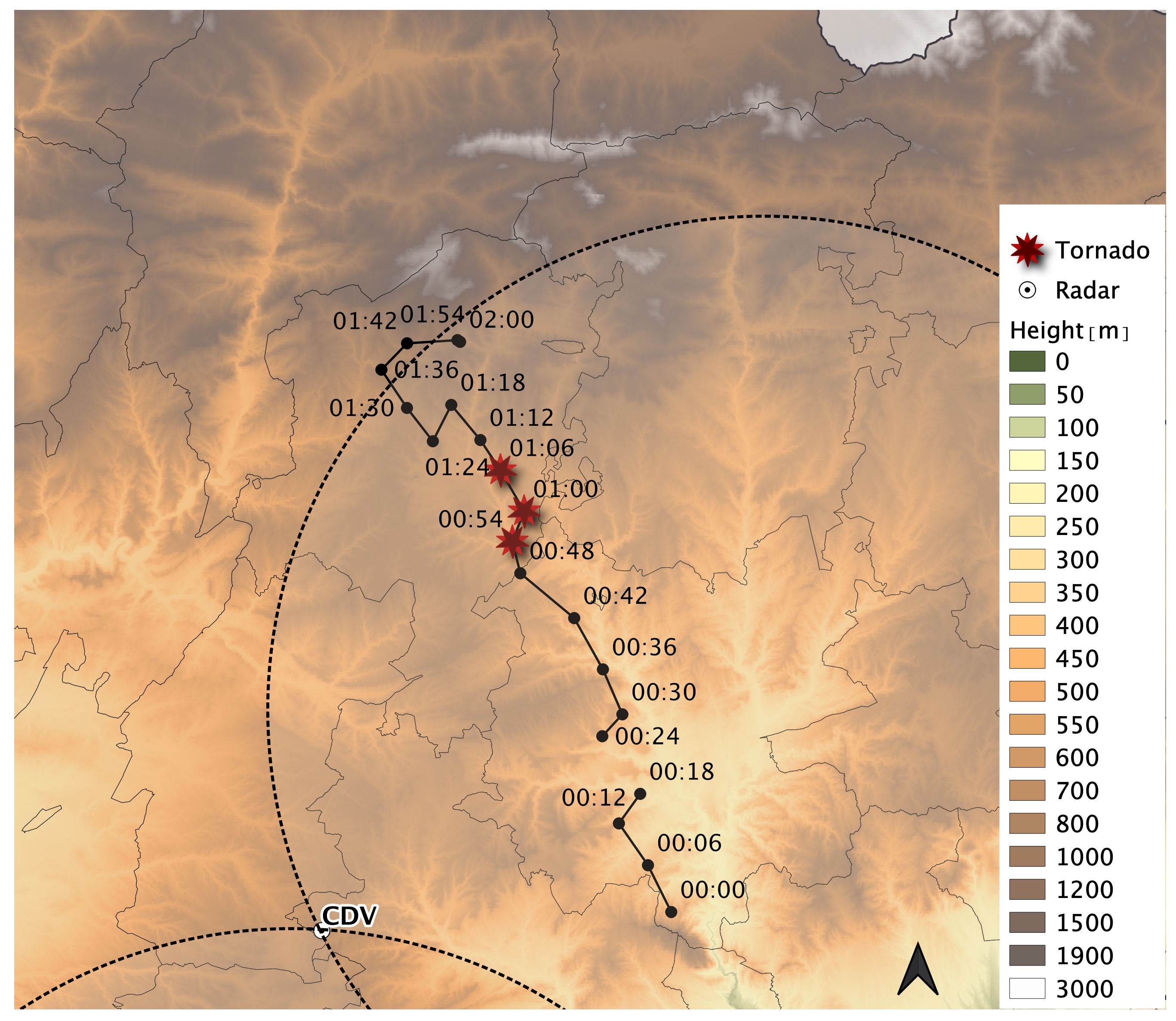
Fig 4: Track of the nocturnal winter storm that produced the tornado on Central Catalonia on 7 January 2018. Part of the 30° CDV-PBE pair dual lobes is depicted in the dotted lines. Dots indicate supercell centroid times labeled in UTC.
Figure 5 shows the CDV radar reflectivity and radial velocity fields for the tornado on January 7, 2018, depicting a hook echo and a mesocyclone, respectively. This is the timestep we will analyse with SAMURAI.
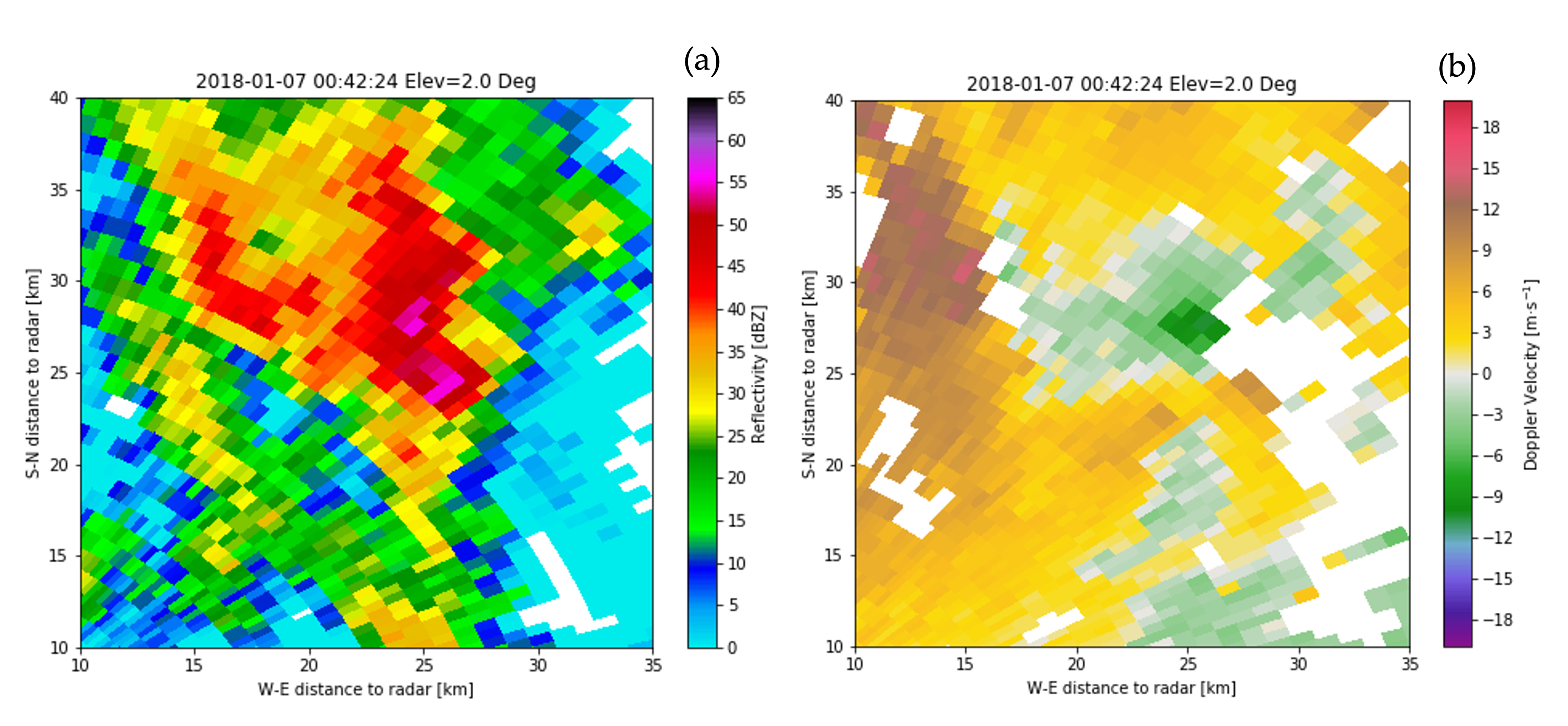
Fig 5: (a) Reflectivity (dBZ) and (b) doppler velocity (m/s) for the supercell case on 7 January 2018 at 0042UTC and 2° elevation angle.
References:
- Armijo, L., 1967. A theory for the determination of wind and precipitation velocities with Doppler radars (Vol. 35). Institutes for Environmental Research, National Severe Storms Laboratory
- Davies-Jones, R.P., 1979. Dual-Doppler radar coverage area as a function of measurement accuracy and spatial resolution. Journal of Applied Meteorology (1962-1982), pp.1229-1233
- del Moral Méndez, A., 2020. Radar-based nowcasting of severe thunderstorms: A better understanding of the dynamical influence of complex topography and the sea
- del Moral Méndez, A.D., Weckwerth, T.M., Rigo, T., Bell, M.M. and Llasat Botija, M.D.C., 2020. C-Band Dual-Doppler Retrievals in Complex Terrain: Improving the Knowledge of Severe Storm Dynamics in Catalonia. Remote Sensing, 2020, vol. 12, num. 18, p. 2930
- Friedrich, K. and Hagen, M., 2004. On the use of advanced Doppler radar techniques to determine horizontal wind fields for operational weather surveillance. Meteorological Applications, 11(2), pp.155-171
- Lhermitte, R.M. and Miller, L.J., 1970. Doppler radar methodology for the observation of convective storms
- Miller, L.J. and Strauch, R.G., 1974. A dual Doppler radar method for the determination of wind velocities within precipitating weather systems. Remote Sensing of Environment, 3(4), pp.219-235
- Rauber, R.M. and Nesbitt, S.W., 2018. Radar meteorology: A first course. John Wiley & Sons
- Ray, P.S. and Sangren, K.L., 1983. Multiple-Doppler radar network design. Journal of climate and applied meteorology, pp.1444-1454
- Ray, P.S. and Wagner, K.K., 1976. Multiple Doppler radar observations of storms. Geophysical Research Letters, 3(3), pp.189-191