In this tutorial, we demonstrate how to exploit GPM-API along with other radar software such xradar and wradlib to match reflectivities measurements of spaceborne (SR) and ground (GR) radars.
We guide you step-by-step through the process of obtaining spatially and temporally coincident radar samples.
The procedure, based on Schwaller and Morris (2011) and adapted by Warren, et. al. (2018), involves:
averaging SR reflectivities vertically along the SR beam between the half-power points of the GR sweep.
averaging GR reflectivities horizontally within the SR beam’s footprint.
The basic principle is illustrated in Fig. 2 of the original paper of Schwaller and Morris (2011).
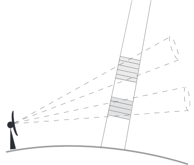
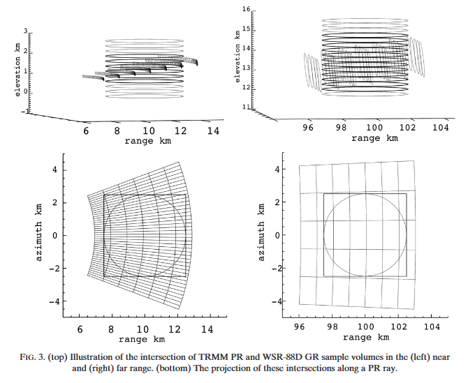
Warren et al. (2018) describe the method as follows: “[...] intersections between individual SR beams and GR elevation sweeps are identified and the reflectivity values from both instruments are averaged within a spatial neighborhood around the intersection. Specifically, SR data are averaged in range over the width of the GR beam at the GR range of the intersection, while GR data are averaged in the range–azimuth plane within the footprint of the SR beam. The result is a pair of reflectivity measurements corresponding to approximately the same volume of atmosphere. [...]”.
The procedure should become clearer in Fig. 3:
In this tutorial, we demonstrate how to exploit GPM-API together with other radar-processing software such xradar and wradlib to match reflectivity measurements from spaceborne radar(SR) and ground-based radar(GR). The matched measurements are then used to assess the calibration bias of the ground radar.
As a case study, we use a GPM Dual-frequency Precipitation Radar (DPR) overpass that captured a convective storm on 12 August 2017 at 17:17:00. The same storm was observed by the Serbian dual-polarization S-band radar of Jastrebac.
To facilitate your hands-on experience, we preprocessed the native Rainbow data from the Serbian radar with xradar and the coincident GPM DPR observations with GPM-API. The resulting datasets were saved in Zarr format and uploaded to a cloud bucket, allowing you to begin the tutorial directly in the Binder environment.
To adapt this workflow to your own case study, use xradar to read your ground-radar data and convert it into the expected xarray format. You can then use GPM-API to retrieve the corresponding GPM observations.
The GPM-API volume_matching routine can also automatically download and open the coincident GPM overpass when an SR dataset is not explicitly provided.
Please read the Spaceborne-Ground Radar Matching Tutorial for a step-by-step guide through the process of obtaining spatially and temporally coincident radar samples.
Now let’s start the tutorial by importing the required packages:
import warnings

warnings.filterwarnings("ignore")

from functools import reduce

import s3fs
import icechunk
import numpy as np
import pandas as pd
import xradar as xd
import xarray as xr
import gpm.gv
import gpm.gv.xradar
import cartopy.crs as ccrs
import matplotlib.pyplot as plt
from IPython.display import display
from xarray.backends.api import open_datatree
from gpm.gv import (
    calibration_summary,
    compare_maps,
    reflectivity_scatterplots,
    volume_matching,
)

np.set_printoptions(suppress=True)
1. Load SR and GR data
Now let’s open the preprocessed GPM DPR dataset composed of the L1B-Ku and 2A-DPR products:
# Open spaceborne radar (SR) GPM DPR dataset (2017-08-12 17:17:00)
ENDPOINT = "https://umn1.osn.mghpcc.org"
STORE = "nexrad-arco/GPM-Data.zarr"
fs = s3fs.S3FileSystem(anon=True, client_kwargs={"endpoint_url": ENDPOINT})
ds_gpm = xr.open_zarr(s3fs.S3Map(STORE, s3=fs), consolidated=False)
ds_gpm = ds_gpm.compute()
Now let’s open the Jastrebac GR data archive
OSN_ENDPOINT = "https://umn1.osn.mghpcc.org"
BUCKET = "nexrad-arco"
prefix = "jastrebac_500m"  # dual-pol, 12 × 360 × 500,  2017 + 2026
root = "JSTB_250_Dp_leto"

storage = icechunk.s3_storage(
    bucket=BUCKET,
    prefix=prefix,
    endpoint_url=OSN_ENDPOINT,
    region="us-east-1",
    anonymous=True,
    force_path_style=True,
)
repo = icechunk.Repository.open(storage)
dt = xr.open_datatree(
    repo.readonly_session("main").store,
    engine="zarr",
    consolidated=False,
    chunks={},
)
dtHere below, we add the radar-site coordinates provided in the DataTree root (longitude, latitude, and altitude) to each sweep dataset to preserve the geolocation information when the sweeps are processed individually later.
for sweep in dt[root].xradar_dev.sweeps:
    node = dt[root][sweep]
    ds = node.to_dataset(inherit=False)
    ds = ds.assign_coords(dt[root].coords) # add latitude/longitude/altitude
    ds = ds.assign_coords(
        sweep_mode="azimuth_surveillance"
    )
    node.dataset = ds
Now, let’s retrieve the time period of the coincident GPM overpass
# Define GPM start_time and end_time
start_time = ds_gpm.gpm.start_time
end_time = ds_gpm.gpm.end_time
print(start_time)
print(end_time)
2017-08-12 17:18:01
2017-08-12 17:18:59
2. Explore GR data
and let’s select the ground radar scan volume and lowest-sweep coincident with the GPM overpass:
# Extract a scan volume coincident with the GPM overpass
dt_gr = dt[root].sel(vcp_time=start_time, method="nearest")

# Extract the lowest sweep
ds_gr = dt_gr["sweep_0"].to_dataset().compute()
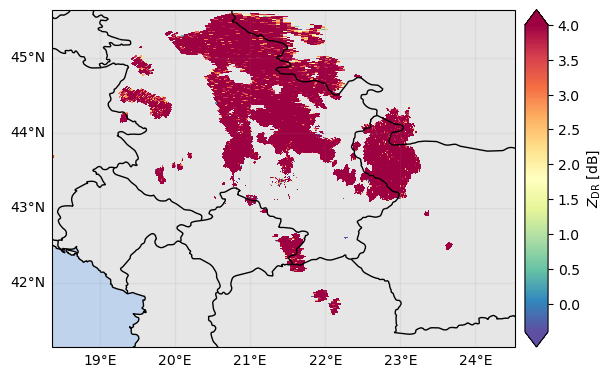
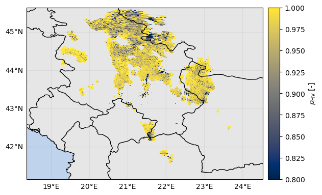
Now we quickly explore the ground radar fields using the xradar_dev.plot_map method:
# Mask non precipitating area
ds_gr = ds_gr.where(ds_gr["DBZH"] > -10).where(ds_gr["RHOHV"] > 0.4)

# Plot fields
ds_gr["DBZH"].xradar_dev.plot_map()
ds_gr["ZDR"].xradar_dev.plot_map()
ds_gr["RHOHV"].xradar_dev.plot_map(vmin=0.8, vmax=1)
<cartopy.mpl.geocollection.GeoQuadMesh at 0x7fae3cda7110>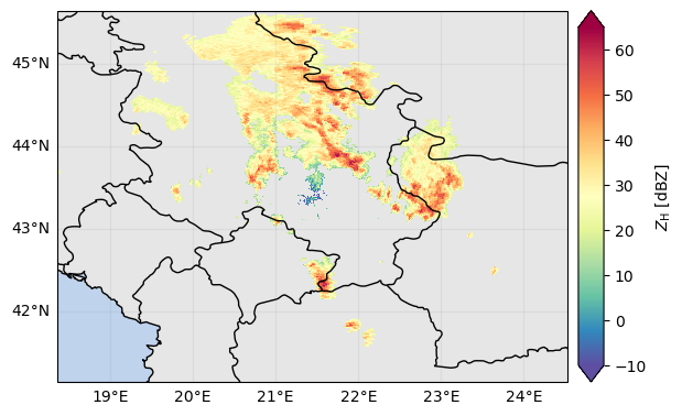
Now let’s restrict the area to 150 km around the ground radar and plot the lowest-sweep S-band measured reflectivity:
# Define extent around radar
extent = ds_gr.xradar_dev.extent(max_distance=150_000)

# Display ground radar reflectivity of lowest sweep
ds_gr["DBZH"].xradar_dev.plot_map(extent=extent)
<cartopy.mpl.geocollection.GeoQuadMesh at 0x7fade972da90>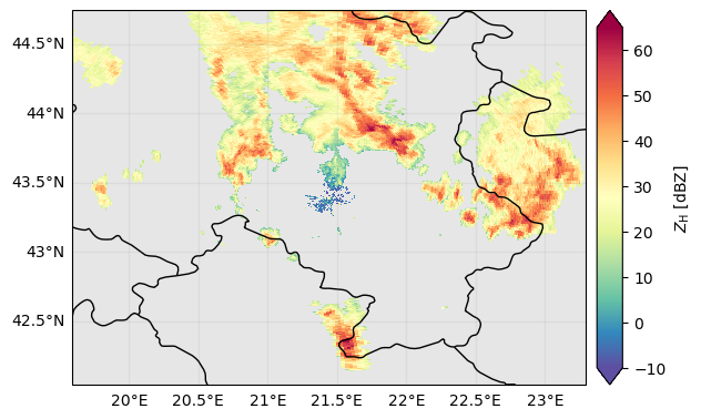
Now let’s display the GPM DPR Ku-band measured reflectivity near the surface just above the surface clutter:
# Display GPM radar reflectivity near the surface
da_gpm_z = ds_gpm["zFactorFinalNearSurface"].sel(radar_frequency="Ku")
p = da_gpm_z.gpm.plot_map()
p.axes.set_extent(extent)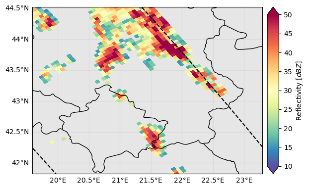
3. Explore GPM DPR data
In this subsection we quickly investigate the GPM DPR data using various GPM-API utilities.
3.1 GPM-API community-based retrievals
GPM-API allows to automatically retrieve various products/quantities through the gpm.retrieve method.
ds_gpm.gpm.available_retrievals() # List of available products/quantities for GPM DPR 2A products['EchoDepth',
'EchoTopHeight',
'HailKineticEnergy',
'MESH',
'MESHS',
'POH',
'POSH',
'REFC',
'REFCH',
'SHI',
'VIL',
'VILD',
'bright_band_ratio',
'c_band_tan',
'dfrFinal',
'dfrFinalNearSurface',
'dfrMeasured',
'flagHydroClass',
'flagPrecipitationType',
'gate_resolution',
'gate_volume',
'heightClutterFreeBottom',
'heightRealSurfaceKa',
'heightRealSurfaceKu',
'range_distance_from_ellipsoid',
'range_distance_from_satellite',
'range_resolution',
's_band_cao2013',
'x_band_tan']We now retrieve the precipitation type and hydrometeor class:
# Retrieve precipitation type and hydrometeor class
ds_gpm["flagPrecipitationType"] = ds_gpm.gpm.retrieve("flagPrecipitationType", method="major_rain_type")
ds_gpm["flagHydroClass"] = ds_gpm.gpm.retrieve("flagHydroClass").sel(radar_frequency="Ku")
3.2 GPM-API visualization tools
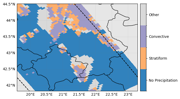
We now display the estimated near surface precipitation rate and precipitation type:
# Display GPM near surface precipitation rate
p = ds_gpm["precipRateNearSurface"].gpm.plot_map()
p.axes.set_extent(extent)

# Investigate precipitation type
p = ds_gpm["flagPrecipitationType"].gpm.plot_map()
p.axes.set_extent(extent)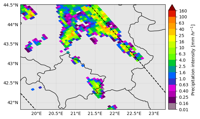
It is always useful to inspect several additional variables. While developing this tutorial, we noticed that, for this particular overpass, the GPM DPR algorithm did not provide values for the attenuation-reliability flag across all scan footprints. Values were missing in the outer portions of the DPR swath. If this issue had gone unnoticed, the subsequent standard calibration routine would have filtered out all footprints in those outer regions.
p = ds_gpm["reliabFlag"].gpm.plot_map()
p.axes.set_extent(extent)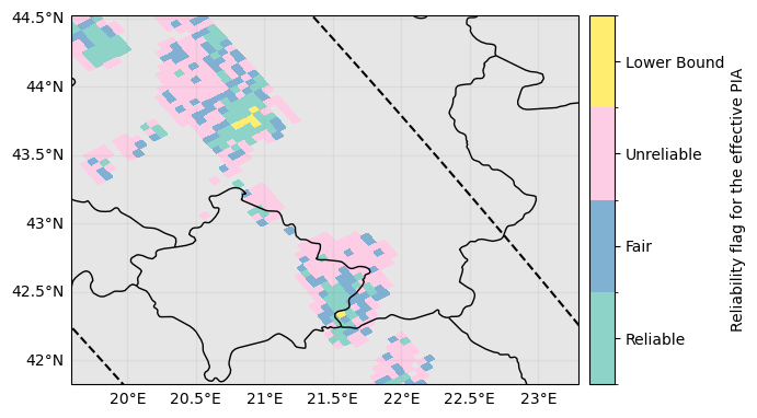
3.3 GPM-API manipulations tools
GPM-API provide a large set of manipulations tools. You can list the available methods with:
display(dir(ds_gpm.gpm))['__class__',
'__delattr__',
'__dict__',
'__dir__',
'__doc__',
'__eq__',
'__firstlineno__',
'__format__',
'__ge__',
'__getattribute__',
'__getstate__',
'__gt__',
'__hash__',
'__init__',
'__init_subclass__',
'__le__',
'__lt__',
'__module__',
'__ne__',
'__new__',
'__reduce__',
'__reduce_ex__',
'__repr__',
'__setattr__',
'__sizeof__',
'__static_attributes__',
'__str__',
'__subclasshook__',
'__weakref__',
'_obj',
'available_retrievals',
'bin_near_surface',
'bin_top',
'bin_variables',
'broadcast_like',
'cartopy_crs',
'collocate',
'crop',
'crop_around_point',
'crop_around_valid_data',
'crop_by_continent',
'crop_by_country',
'cross_section_variables',
'end_time',
'extent',
'extract_at_points',
'extract_dataset_above_bin',
'extract_dataset_below_bin',
'extract_l2_dataset',
'extract_transect_along_dimension',
'extract_transect_around_point',
'extract_transect_at_points',
'extract_transect_between_points',
'frequency_variables',
'get_crop_slices_around_point',
'get_crop_slices_by_continent',
'get_crop_slices_by_country',
'get_crop_slices_by_extent',
'get_height_at_bin',
'get_slices_contiguous_granules',
'get_slices_contiguous_scans',
'get_slices_regular',
'get_slices_regular_time',
'get_slices_valid_geolocation',
'has_contiguous_scans',
'has_missing_granules',
'has_regular_time',
'has_valid_geolocation',
'infill_below_bin',
'is_grid',
'is_orbit',
'is_regular',
'is_spatial_2d',
'is_spatial_3d',
'isel',
'mask_above_bin',
'mask_below_bin',
'mask_between_bins',
'plot_cross_section',
'plot_image',
'plot_map',
'plot_map_mesh',
'plot_map_mesh_centroids',
'plot_swath',
'plot_swath_lines',
'plot_transect_line',
'pyproj_crs',
'pyresample_area',
'quadmesh_centroids',
'quadmesh_corners',
'quadmesh_polygons',
'quadmesh_vertices',
'remap_era5',
'remap_on',
'retrieve',
'sel',
'select_bin_variables',
'select_cross_section_variables',
'select_frequency_variables',
'select_spatial_2d_variables',
'select_spatial_3d_variables',
'select_vertical_variables',
'set_crs',
'set_encoding',
'slice_range_at_bin',
'slice_range_at_cfb',
'slice_range_at_height',
'slice_range_at_max_value',
'slice_range_at_min_value',
'slice_range_at_near_surface',
'slice_range_at_surface',
'slice_range_at_temperature',
'slice_range_at_top',
'slice_range_at_value',
'spatial_2d_variables',
'spatial_3d_variables',
'spatial_coordinates',
'spatial_dimensions',
'start_time',
'subset_by_time',
'subset_by_time_slice',
'subset_range_by_height',
'subset_range_where_values',
'subset_range_with_valid_data',
'title',
'to_dask_dataframe',
'to_pandas_dataframe',
'unstack_dimension',
'variables',
'vertical_dimension',
'vertical_variables',
'x',
'y']We now analyze the hydrometeor class at various heights:
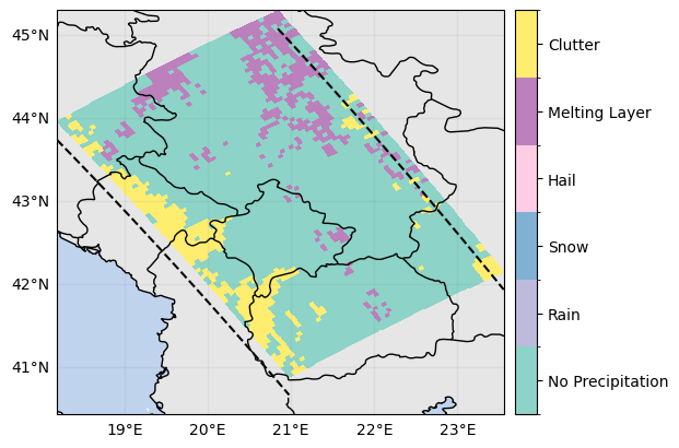
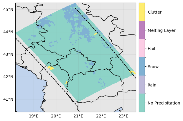
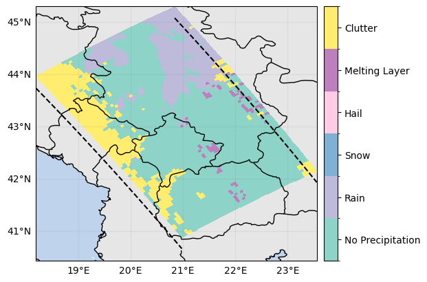
ds_gpm.gpm.slice_range_at_bin(bins="binClutterFreeBottom")["flagHydroClass"].gpm.plot_map()<cartopy.mpl.geocollection.GeoQuadMesh at 0x7fadeb70ad50>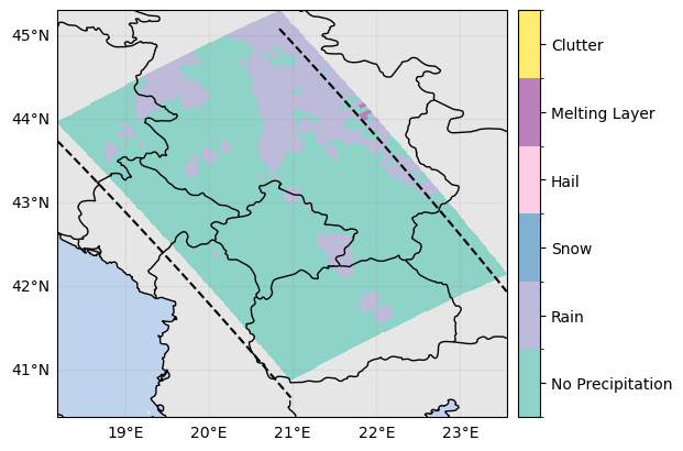
ds_gpm.gpm.slice_range_at_height(2000)["flagHydroClass"].gpm.plot_map()
ds_gpm.gpm.slice_range_at_height(3000)["flagHydroClass"].gpm.plot_map()
ds_gpm.gpm.slice_range_at_height(4000)["flagHydroClass"].gpm.plot_map()
<cartopy.mpl.geocollection.GeoQuadMesh at 0x7fadeb138550>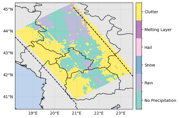
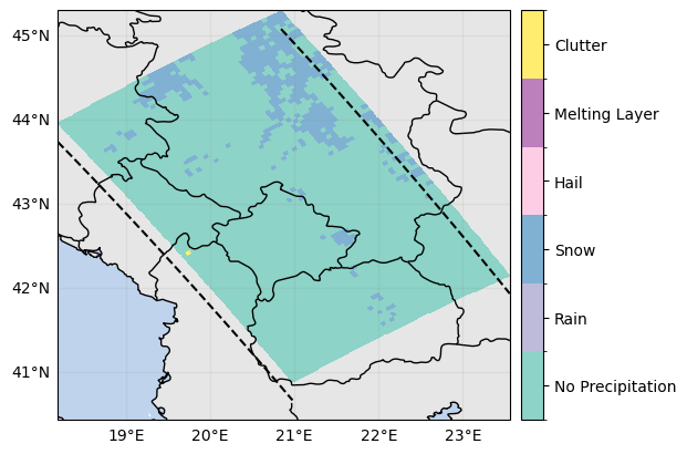
ds_gpm.gpm.slice_range_at_temperature(temperature=275.15)["flagHydroClass"].gpm.plot_map()
ds_gpm.gpm.slice_range_at_temperature(temperature=275.15-5)["flagHydroClass"].gpm.plot_map()
ds_gpm.gpm.slice_range_at_temperature(temperature=275.15+5)["flagHydroClass"].gpm.plot_map()
<cartopy.mpl.geocollection.GeoQuadMesh at 0x7fadeb0cc190>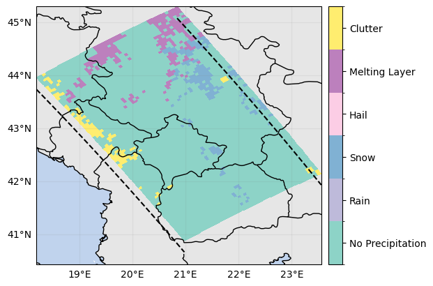
ds_gpm["flagHydroClass"].sel(range=[165, 160, 155, 150]).gpm.plot_map(col="range", col_wrap=2)<gpm.visualization.facetgrid.CartopyFacetGrid at 0x7fadf0467230>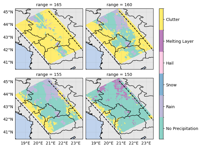
The first clutter free gate is located at such heights:
ds_gpm.gpm.get_height_at_bin("binClutterFreeBottom").gpm.plot_map()<cartopy.mpl.geocollection.GeoQuadMesh at 0x7fadead61bd0>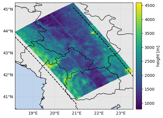
The approximate surface elevation can be illustrated using the binRealSurface variable:
ds_gpm.sel(radar_frequency="Ku").gpm.get_height_at_bin("binRealSurface").gpm.plot_map()<cartopy.mpl.geocollection.GeoQuadMesh at 0x7fadead9b890>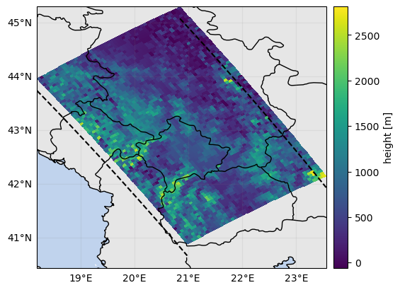
3.4 GPM-API vertical cross-sections
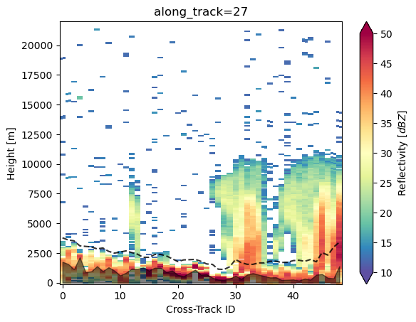
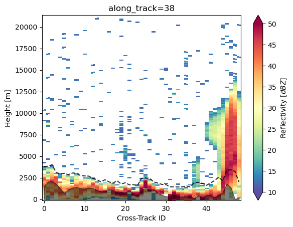
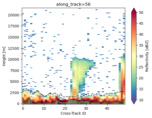
Here below, we provide the code to plot cross sections of the measured reflectivity along all or selected GPM DPR scans. The dashed line marks the gates located above the surface-clutter zone, while the shaded region below represents the actual surface.
indices = range(ds_gpm.sizes["along_track"])
indices = [0, 27, 38, 56] # comment this to loop over all scans
for i in indices:
    ds_transect = ds_gpm.sel(radar_frequency="Ku").isel(along_track=i)
    da_height_free_clutter = ds_transect.gpm.get_height_at_bin("binClutterFreeBottom")
    da_height_surface = ds_transect.gpm.get_height_at_bin("binRealSurface")
    ds_transect["zFactorMeasured"] = ds_transect["zFactorMeasured"].where(ds_transect["zFactorMeasured"] > 12)
    p = ds_transect["zFactorMeasured"].gpm.plot_cross_section()
    da_height_free_clutter.plot.line(ax=p.axes, c="black", alpha=0.8, linestyle="--")
    p.axes.fill_between(
        x=da_height_surface["cross_track"],
        y1=da_height_surface,
        y2=0,
        color="black",
        alpha=0.5,
    )
    p.axes.set_xlabel("Cross-Track ID")
    p.axes.set_ylabel("Height [m]")
    p.axes.set_title(f"along_track={i}")
    plt.show()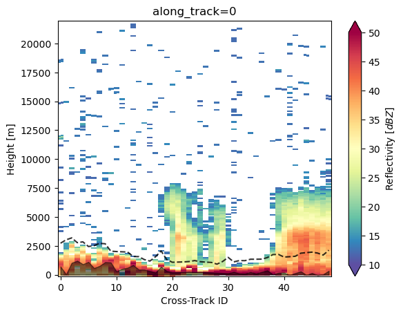
4. Volume matching of a GR sweep to coincident SR footprints
Here we start defining the required settings for the SR/GR volume matching procedure:
The GR
radar_bandcontrols to which frequency SR Ku-band reflectivities will be converted. Valid values areX,C,S,Ku.The
beamwidth_grrefers to the angular beam width of the GR.The minimum reflectivity thresholds
z_min_threshold_srandz_min_threshold_grare used to mask out SR and GR gates belows such thresholds.
# Define GR-GPM volume matching settings
radar_band = "S"
beamwidth_gr = 1
z_min_threshold_gr = 0
z_min_threshold_sr = 10
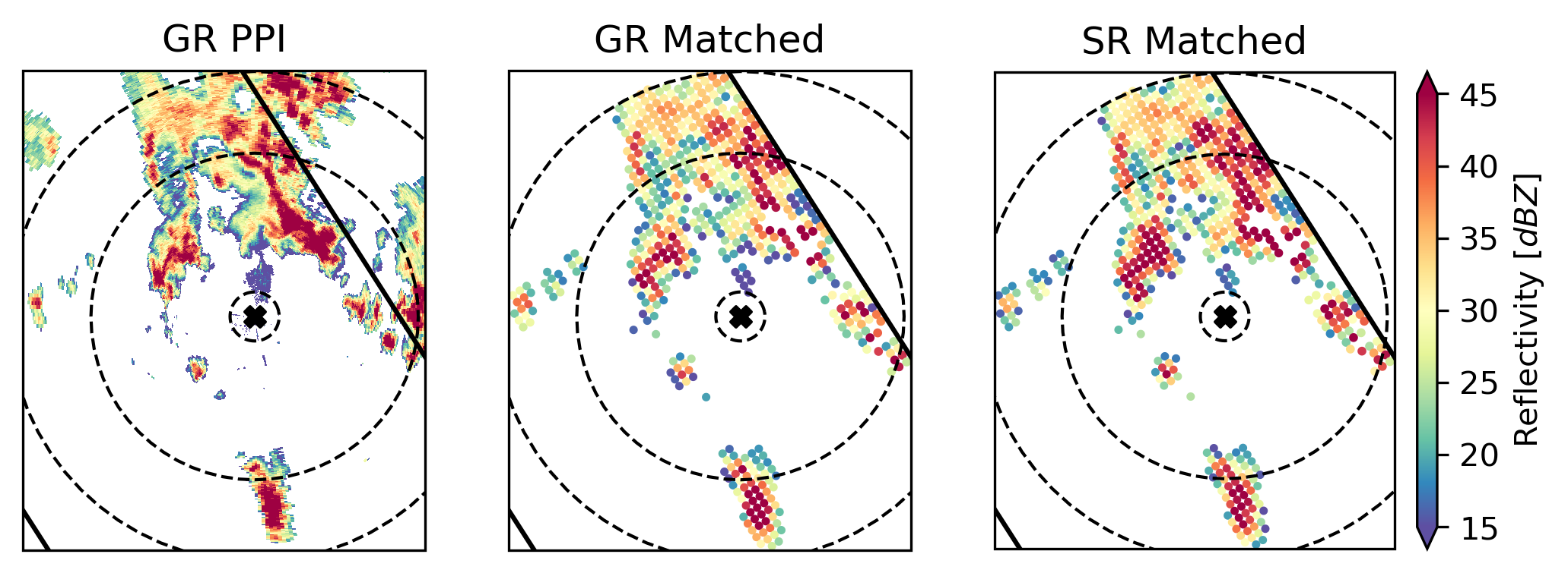
The SR/GR volume matching routine typically takes a few seconds to complete. It returns a geopandas.DataFrame with the matched aggregated reflectivities and the associated statistics.
# Match GR sweep to GPM footprints
gdf_match = volume_matching(
    ds_gr=ds_gr,
    ds_sr=ds_gpm,
    z_variable_gr="DBZH",
    radar_band=radar_band,
    beamwidth_gr=beamwidth_gr,
    z_min_threshold_gr=z_min_threshold_gr,
    z_min_threshold_sr=z_min_threshold_sr,
    min_gr_range=0,
    max_gr_range=150_000,
    download_sr=False,  # require internet connection !
    display_quicklook=True,
    display_calibration_summary=True,

)
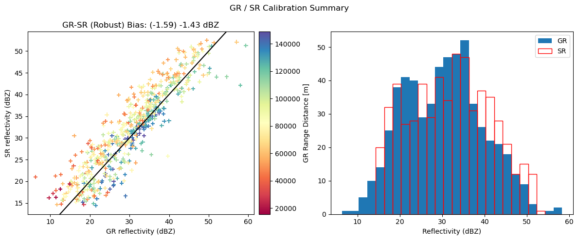
SR/GR Matching Elapsed time: 0:00:04.666478 .
display(gdf_match)The variables included in the SR/GR database are listed here below:
# List variables
display(list(gdf_match))
['GR_time',
'GR_gate_volume_sum',
'GR_fraction_covered_area',
'GR_counts',
'GR_counts_valid',
'geometry',
'GR_range_max',
'GR_range_mean',
'GR_range_min',
'GR_azimuth',
'GR_elevation',
'GR_Z_fraction_above_10dBZ',
'GR_Z_fraction_above_12dBZ',
'GR_Z_fraction_above_14dBZ',
'GR_Z_fraction_above_16dBZ',
'GR_Z_fraction_above_18dBZ',
'distance_horizontal_min',
'distance_horizontal_mean',
'distance_horizontal_max',
'GR_Z_cumsum_mean',
'GR_Z_cumsum_min',
'GR_Z_cumsum_max',
'GR_Z_cumsum_std',
'GR_Z_cumsum_range',
'GR_Z_cumsum_cov',
'GR_gate_volume_mean',
'GR_gate_volume_min',
'GR_gate_volume_max',
'GR_gate_volume_std',
'GR_gate_volume_range',
'GR_gate_volume_cov',
'GR_hres_mean',
'GR_hres_min',
'GR_hres_max',
'GR_hres_std',
'GR_hres_range',
'GR_hres_cov',
'GR_vres_mean',
'GR_vres_min',
'GR_vres_max',
'GR_vres_std',
'GR_vres_range',
'GR_vres_cov',
'GR_x_mean',
'GR_x_min',
'GR_x_max',
'GR_x_std',
'GR_x_range',
'GR_x_cov',
'GR_y_mean',
'GR_y_min',
'GR_y_max',
'GR_y_std',
'GR_y_range',
'GR_y_cov',
'GR_z_mean',
'GR_z_min',
'GR_z_max',
'GR_z_std',
'GR_z_range',
'GR_z_cov',
'GR_DBZH_mean',
'GR_DBZH_min',
'GR_DBZH_max',
'GR_DBZH_std',
'GR_DBZH_range',
'GR_DBZH_cov',
'GR_Z_mean',
'GR_Z_std',
'GR_Z_max',
'GR_Z_min',
'GR_Z_range',
'GR_Z_cov',
'SR_counts',
'SR_counts_valid',
'SR_zFactorFinal_Ku_fraction_above_10dBZ',
'SR_zFactorFinal_Ku_fraction_above_12dBZ',
'SR_zFactorFinal_Ku_fraction_above_14dBZ',
'SR_zFactorFinal_Ku_fraction_above_16dBZ',
'SR_zFactorFinal_Ku_fraction_above_18dBZ',
'SR_zFactorFinal_S_fraction_above_10dBZ',
'SR_zFactorFinal_S_fraction_above_12dBZ',
'SR_zFactorFinal_S_fraction_above_14dBZ',
'SR_zFactorFinal_S_fraction_above_16dBZ',
'SR_zFactorFinal_S_fraction_above_18dBZ',
'SR_zFactorMeasured_Ku_fraction_above_10dBZ',
'SR_zFactorMeasured_Ku_fraction_above_12dBZ',
'SR_zFactorMeasured_Ku_fraction_above_14dBZ',
'SR_zFactorMeasured_Ku_fraction_above_16dBZ',
'SR_zFactorMeasured_Ku_fraction_above_18dBZ',
'SR_zFactorMeasured_S_fraction_above_10dBZ',
'SR_zFactorMeasured_S_fraction_above_12dBZ',
'SR_zFactorMeasured_S_fraction_above_14dBZ',
'SR_zFactorMeasured_S_fraction_above_16dBZ',
'SR_zFactorMeasured_S_fraction_above_18dBZ',
'SR_PIA_Ku_mean',
'SR_airTemperature_mean',
'SR_gate_volume_mean',
'SR_hres_mean',
'SR_precipRate_mean',
'SR_vres_mean',
'SR_x_mean',
'SR_y_mean',
'SR_z_mean',
'SR_zFactorCorrection_Ku_mean',
'SR_zFactorCorrection_S_mean',
'SR_zFactorFinal_Ku_mean',
'SR_zFactorFinal_Ku_cumsum_mean',
'SR_zFactorFinal_S_mean',
'SR_zFactorFinal_S_cumsum_mean',
'SR_zFactorMeasured_Ku_mean',
'SR_zFactorMeasured_Ku_cumsum_mean',
'SR_zFactorMeasured_S_mean',
'SR_zFactorMeasured_S_cumsum_mean',
'SR_PIA_Ku_std',
'SR_airTemperature_std',
'SR_gate_volume_std',
'SR_hres_std',
'SR_precipRate_std',
'SR_vres_std',
'SR_x_std',
'SR_y_std',
'SR_z_std',
'SR_zFactorCorrection_Ku_std',
'SR_zFactorCorrection_S_std',
'SR_zFactorFinal_Ku_std',
'SR_zFactorFinal_Ku_cumsum_std',
'SR_zFactorFinal_S_std',
'SR_zFactorFinal_S_cumsum_std',
'SR_zFactorMeasured_Ku_std',
'SR_zFactorMeasured_Ku_cumsum_std',
'SR_zFactorMeasured_S_std',
'SR_zFactorMeasured_S_cumsum_std',
'SR_PIA_Ku_sum',
'SR_airTemperature_sum',
'SR_gate_volume_sum',
'SR_hres_sum',
'SR_precipRate_sum',
'SR_vres_sum',
'SR_x_sum',
'SR_y_sum',
'SR_z_sum',
'SR_zFactorCorrection_Ku_sum',
'SR_zFactorCorrection_S_sum',
'SR_zFactorFinal_Ku_sum',
'SR_zFactorFinal_Ku_cumsum_sum',
'SR_zFactorFinal_S_sum',
'SR_zFactorFinal_S_cumsum_sum',
'SR_zFactorMeasured_Ku_sum',
'SR_zFactorMeasured_Ku_cumsum_sum',
'SR_zFactorMeasured_S_sum',
'SR_zFactorMeasured_S_cumsum_sum',
'SR_PIA_Ku_max',
'SR_airTemperature_max',
'SR_gate_volume_max',
'SR_hres_max',
'SR_precipRate_max',
'SR_vres_max',
'SR_x_max',
'SR_y_max',
'SR_z_max',
'SR_zFactorCorrection_Ku_max',
'SR_zFactorCorrection_S_max',
'SR_zFactorFinal_Ku_max',
'SR_zFactorFinal_Ku_cumsum_max',
'SR_zFactorFinal_S_max',
'SR_zFactorFinal_S_cumsum_max',
'SR_zFactorMeasured_Ku_max',
'SR_zFactorMeasured_Ku_cumsum_max',
'SR_zFactorMeasured_S_max',
'SR_zFactorMeasured_S_cumsum_max',
'SR_PIA_Ku_min',
'SR_airTemperature_min',
'SR_gate_volume_min',
'SR_hres_min',
'SR_precipRate_min',
'SR_vres_min',
'SR_x_min',
'SR_y_min',
'SR_z_min',
'SR_zFactorCorrection_Ku_min',
'SR_zFactorCorrection_S_min',
'SR_zFactorFinal_Ku_min',
'SR_zFactorFinal_Ku_cumsum_min',
'SR_zFactorFinal_S_min',
'SR_zFactorFinal_S_cumsum_min',
'SR_zFactorMeasured_Ku_min',
'SR_zFactorMeasured_Ku_cumsum_min',
'SR_zFactorMeasured_S_min',
'SR_zFactorMeasured_S_cumsum_min',
'SR_PIA_Ku_range',
'SR_airTemperature_range',
'SR_gate_volume_range',
'SR_hres_range',
'SR_precipRate_range',
'SR_vres_range',
'SR_x_range',
'SR_y_range',
'SR_z_range',
'SR_zFactorCorrection_Ku_range',
'SR_zFactorCorrection_S_range',
'SR_zFactorFinal_Ku_range',
'SR_zFactorFinal_Ku_cumsum_range',
'SR_zFactorFinal_S_range',
'SR_zFactorFinal_S_cumsum_range',
'SR_zFactorMeasured_Ku_range',
'SR_zFactorMeasured_Ku_cumsum_range',
'SR_zFactorMeasured_S_range',
'SR_zFactorMeasured_S_cumsum_range',
'SR_fraction_no_precip',
'SR_fraction_rain',
'SR_fraction_snow',
'SR_fraction_hail',
'SR_fraction_melting_layer',
'SR_fraction_clutter',
'SR_fraction_below_isotherm',
'SR_fraction_above_isotherm',
'SR_flagPrecip',
'SR_flagPrecipitationType',
'SR_dataQuality',
'SR_sunLocalTime',
'SR_SCorientation',
'SR_qualityFlag',
'SR_qualityTypePrecip',
'SR_qualityBB',
'SR_pathAtten',
'SR_piaFinal',
'SR_reliabFlag',
'SR_time',
'gpm_along_track_id',
'gpm_cross_track_id',
'gpm_granule_id',
'gpm_id',
'lat',
'lon',
'sweep_fixed_angle',
'VolumeRatio',
'VolumeDiff',
'time_difference',
'GR_z_lower_bound',
'GR_z_upper_bound',
'SR_z_lower_bound',
'SR_z_upper_bound']5. Explore the SR/GR database
Now let’s analyse the SR/GR reflectivities of a single sweep:
sr_z_column = f"SR_zFactorFinal_{radar_band}_mean"
gr_z_column = "GR_Z_mean"
We start by comparing the spatial reflectivity fields without applying restrictive filtering criteria:
fig = compare_maps(
    gdf_match,
    sr_column=sr_z_column,
    gr_column=gr_z_column,
    sr_label="SR Reflectivity (dBz)",
    gr_label="GR Reflectivity (dBz)",
    cmap="Spectral_r",
    unified_color_scale=True,
    vmin=15,
    # vmax=40
)
fig.tight_layout()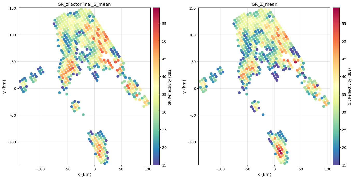
If you wish to create a cartopy map, specify the 'projection' in the subplot_kwargs argument:
ccrs_gr_aeqd = ccrs.AzimuthalEquidistant(
    central_longitude=ds_gr["longitude"].item(),
    central_latitude=ds_gr["latitude"].item(),
)
subplot_kwargs = {}
subplot_kwargs["projection"] = ccrs_gr_aeqd
fig = compare_maps(
    gdf_match,
    sr_column=sr_z_column,
    gr_column=gr_z_column,
    sr_label="SR Reflectivity (dBz)",
    gr_label="GR Reflectivity (dBz)",
    cmap="Spectral_r",
    unified_color_scale=True,
    vmin=15,
    # vmax=40
    subplot_kwargs=subplot_kwargs,
)
fig.tight_layout()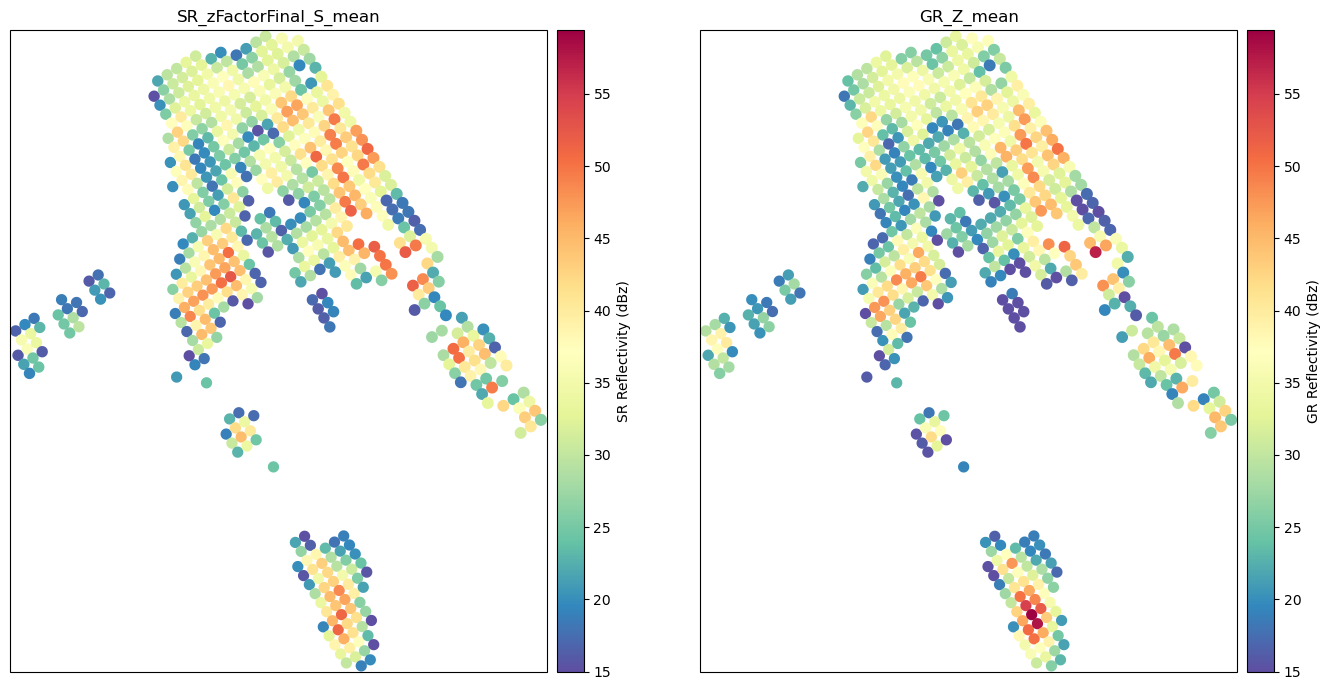
Here we show how to explore interactively the reflectivity fields using Folium:
gdf_match.explore(column="GR_Z_mean", legend=True, cmap="Spectral_r", vmin=0, vmax=40)We now create a figure comparing SR/GR aggregated reflectivities volume-by-volume and displaying the overall distributions.
fig = calibration_summary(
    df=gdf_match,
    gr_z_column=gr_z_column,
    sr_z_column=sr_z_column,
    # Histogram options
    bin_width=2,
    # Scatterplot options
    hue_column="SR_fraction_clutter",
    marker="+",
    cmap="Spectral",
)
fig.tight_layout()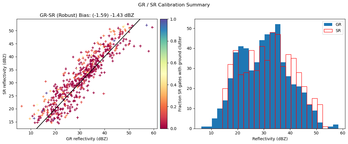
6. Explore SR/GR database filtering criteria
When comparing SR and GR data or trying to determine an accurate GR calibration bias, it’s necessary to define a set of filtering criteria. In the figures below, we perform exploratory data analysis to investigate the relationships between the SR/GR reflectivity deviations and sets of variables characterizing radar measurements and SR/GR volume properties. The patterns and deviations observed in the scatterplots will be used to define a set of filtering criteria in the next section of the tutorial.
hue_columns = [
    "SR_fraction_clutter",
    "SR_fraction_rain",
    "SR_fraction_snow",
    "SR_fraction_hail",
    "SR_fraction_melting_layer",
    "SR_fraction_no_precip",
    "GR_range_max",
    "SR_gate_volume_sum"
]
fig = reflectivity_scatterplots(
    df=gdf_match,
    gr_z_column=gr_z_column,
    sr_z_column=sr_z_column,
    hue_columns=hue_columns,
    ncols=2,
)
fig.tight_layout()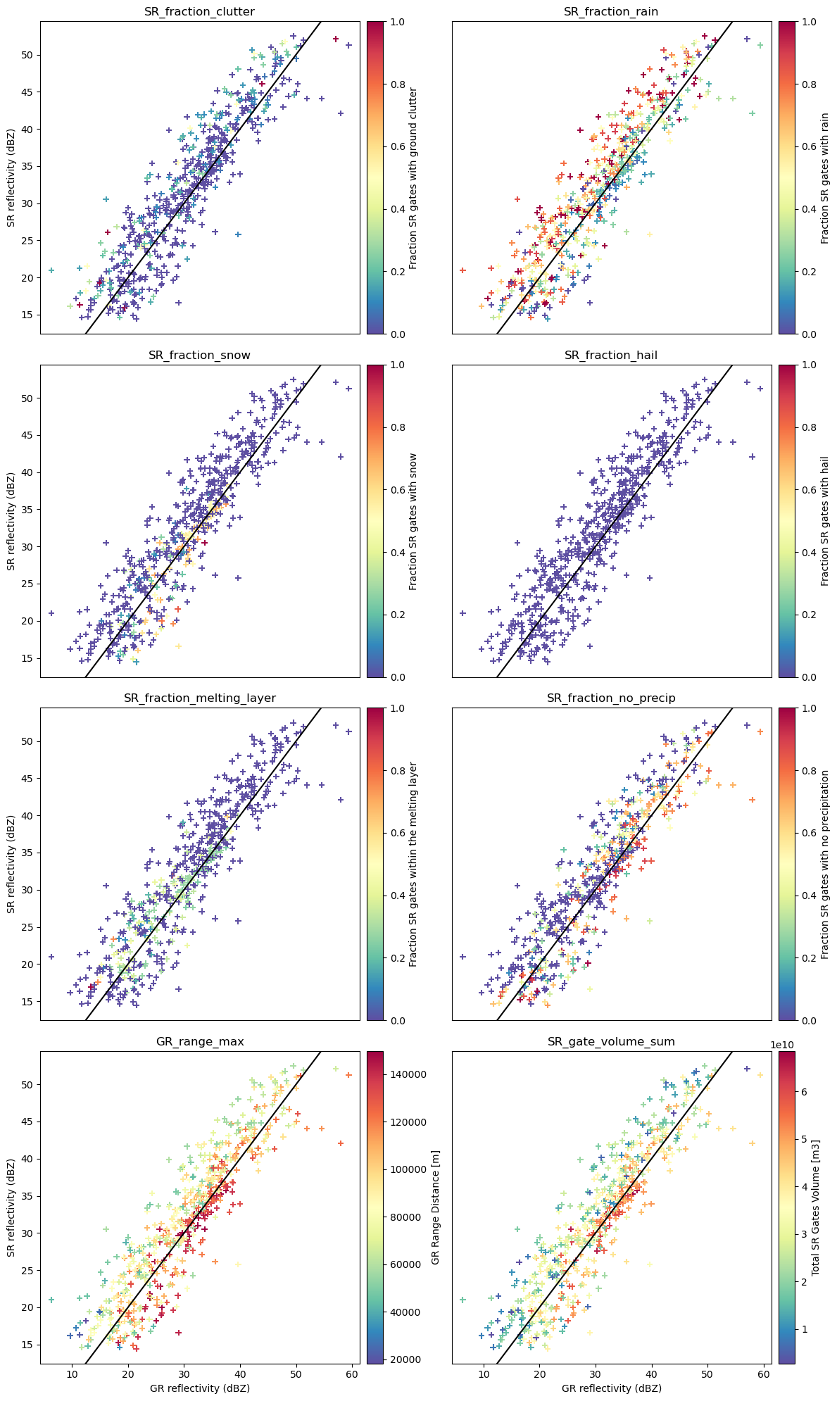
7. Run SR/GR volume matching across sweeps
We will now run the SR/GR volume matching routine to each sweep acquired by the ground radar within 3 minutes from the GPM overpass, and collect the results into a single database
# Select ground radars VCPs within 10 minutes from overpass
search_start = pd.Timestamp(start_time) - pd.Timedelta(10, unit="minutes")
search_end = pd.Timestamp(end_time) + pd.Timedelta(10, unit="minutes")
dt_gr_volumes = dt[root].sel(vcp_time=slice(search_start, search_end))

# Collect VCP sweeps within 3 minutes from GPM DPR overpass
dict_ds_gr = {}
for i in range(dt_gr_volumes.sizes["vcp_time"]):
    # Select VCP
    dt_gr = dt_gr_volumes.isel(vcp_time=i)

    # Process sweeps within 3 minutes from overpass
    search_start = pd.Timestamp(start_time) - pd.Timedelta(3, unit="minutes")
    search_end = pd.Timestamp(end_time) + pd.Timedelta(3, unit="minutes")

    # Loop over VCP sweeps
    for sweep_group in dt_gr.xradar_dev.sweeps:

        # Extract sweep dataset
        ds_gr = dt_gr[sweep_group].to_dataset()

        # Define sweep start and end time
        ds_gr["time"] = ds_gr["time"].compute()
        sweep_start_time = pd.Timestamp(ds_gr["time"].min(skipna=True).to_numpy().item())
        sweep_end_time = pd.Timestamp(ds_gr["time"].max(skipna=True).to_numpy().item())

        # If the sweep has been acquired 3 minutes apart from SR overpass,
        # - do not process the sweep
        no_overlap = (sweep_end_time < search_start) or (sweep_start_time > search_end)
        if no_overlap:
            continue

        # Otherwise process and collect the sweep
        try:
            sweep_idx = int(sweep_group.replace("sweep_", ""))
            time_str = sweep_start_time.strftime("%Y%m%d%H%M%S")
            identifier = f"{time_str}_{sweep_group}"
            dict_ds_gr[identifier] = ds_gr
        except Exception as e:
            if "No variable named" in str(e):
                continue
            print(f"Error while opening {sweep_group} at {time_str} : {str(e)}")
            continue

n_sweeps = len(dict_ds_gr)
print(f"{n_sweeps} sweeps selected for matching with GPM DPR")
19 sweeps selected for matching with GPM DPR
# Define GR/SR volume matching setting
radar_band = "S"
beamwidth_gr = 1
z_min_threshold_gr = 0
z_min_threshold_sr = 10
min_gr_range = 0
max_gr_range = 150_000
z_variable_gr="DBZH"
display_quicklook=True
download_sr=False
gr_sensitivity_thresholds=None
sr_sensitivity_thresholds=None
# Perform volume matching for each GR sweep
# - This typically takes few seconds per sweep to complete
list_gdf = []
for identifier, ds_gr in dict_ds_gr.items():
try:
#---------------------------------------------------------------------.
#### Matching with ground radar
gdf_match = volume_matching(
ds_gr = ds_gr,
ds_sr = ds_gpm,
z_variable_gr=z_variable_gr,
radar_band=radar_band,
beamwidth_gr=beamwidth_gr,
z_min_threshold_gr=z_min_threshold_gr,
z_min_threshold_sr=z_min_threshold_sr,
min_gr_range=min_gr_range,
max_gr_range=max_gr_range,
download_sr=False, # require internet connection !
display_quicklook=False,
)
except Exception as e:
print(f"Volume matching error at {start_time}: {str(e)}")
continue
# Append matching database
if gdf_match is not None:
gdf_match["identifier"] = identifier
gdf_match["sweep_group"] = identifier.split("_", 1)[1]
list_gdf.append(gdf_match)
gdf_match = pd.concat(list_gdf)SR/GR Matching Elapsed time: 0:00:02.361061 .
SR/GR Matching Elapsed time: 0:00:00.853719 .
SR/GR Matching Elapsed time: 0:00:00.748465 .
SR/GR Matching Elapsed time: 0:00:02.628092 .
SR/GR Matching Elapsed time: 0:00:02.522035 .
SR/GR Matching Elapsed time: 0:00:02.623942 .
SR/GR Matching Elapsed time: 0:00:01.612770 .
SR/GR Matching Elapsed time: 0:00:02.862650 .
SR/GR Matching Elapsed time: 0:00:01.705917 .
SR/GR Matching Elapsed time: 0:00:00.865470 .
SR/GR Matching Elapsed time: 0:00:01.579338 .
SR/GR Matching Elapsed time: 0:00:01.057004 .
SR/GR Matching Elapsed time: 0:00:02.170679 .
SR/GR Matching Elapsed time: 0:00:02.634889 .
SR/GR Matching Elapsed time: 0:00:02.575053 .
SR/GR Matching Elapsed time: 0:00:02.628786 .
SR/GR Matching Elapsed time: 0:00:01.661626 .
SR/GR Matching Elapsed time: 0:00:02.739996 .
SR/GR Matching Elapsed time: 0:00:01.296581 .
8. Define SR/GR filtering criteria
When calibrating or comparing SR and GR data, there is a necessary tradeoff between the strictness of filtering criteria filtering and the number of available samples. Here below we provide some general recommendations for effective filtering:
Sensitivity Thresholds: Retain only those radar beams where the aggregated gate reflectivities exceed the instrument sensitivities. The
GR_Z_fraction_above_<thr>dBZandSR_zFactorFinal_Ku_fraction_above_<thr>dBZvariables can be used filter the samples.Stratiform Precipitation: If the purpose of your analysis is to assess the calibration bias of GR data, it is suggested to focus on stratiform precipitation that occurs outside the melting layer (i.e. avoiding the bright band). Only stratiform samples above the melting layer are used in ground validation of the GPM DPR (W. Petersen 2017, personal communication). Convective SR footprints are typically excluded to avoid dealing with:
the high spatial variability in the precipitation field and issues with non-uniform beam filling (NUBF),
the potential biases introduced by the SR attenuation correction,
the potential biases in GR reflectivities, especially at C and X band, due to beam attenuation,
the multiple scattering signature caused by hail particles.
Reflectivity Range: According to Warren et al. (2018), volume-averaged SR and GR reflectivity values should be selected within the range of 24 to 36 dBZ. This range minimizes the impact of low SR sensitivity, SR beam attenuation and non-rayleigh scattering effects.
Clutter Removal: Exclude SR/GR samples that are contaminated by ground clutter, anomalous propagation, or beam blockage.
Volume matching: Exclude SR/GR samples where there are excessive differences in the total gate volume.
def filter_matched_volumes(gdf_match,
                           radar_band,
                           sr_z_range=(18, 36),
                           gr_z_range=(18, 36),
                           display_mask=False):
    # Define masks
    masks = [
        # Select SR scan with "normal" dataQuality (for entire cross-track scan)
        gdf_match["SR_dataQuality"] == 0,
        # Select SR beams with detected precipitation
        gdf_match["SR_flagPrecip"] > 0,
        # Select only 'high quality' SR data
        # - qualityFlag == 1 indicates low quality retrievals
        # - qualityFlag == 2 indicates bad/missing retrievals
        gdf_match["SR_qualityFlag"] == 0,
        # Select only beams with confident precipitation type
        gdf_match["SR_qualityTypePrecip"] == 1,

        # Select only SR beams with detected bright band
        # gdf_match["SR_qualityBB"] == 1,
        # Select only stratiform precipitation
        # - SR_flagPrecipitationType == 2 indicates convective
        # gdf_match["SR_flagPrecipitationType"] == 1,

        # Select only SR beams with reliable attenuation correction
        # --> Buggy values for this event ! Not used
        # gdf_match["SR_reliabFlag"].isin((1, 2)),  # or == 1

        # Select only beams with reduced path attenuation
        # gdf_match["SR_zFactorCorrection_Ku_max"]
        # gdf_match["SR_piaFinal"]
        # gdf_match["SR_pathAtten"]

        # Select only SR beams with matching SR gates with precipitation
        gdf_match["SR_fraction_no_precip"] < 0.1,

        # Select only SR beams with matching SR gates with no clutter
        gdf_match["SR_fraction_clutter"] < 0.05,
        # Select only SR beams with matching SR gates not in the melting layer
        gdf_match["SR_fraction_melting_layer"] < 0.1,
        # Select only SR beams with matching SR gates with no hail
        gdf_match["SR_fraction_hail"] == 0,

        # Select SR beams only within given GR radius interval
        # - Crisologo et al., 2018, Warren et al., 2018
        gdf_match["GR_range_min"] > 15_000,
        gdf_match["GR_range_max"] < 115_000,

        # Discard SR beams where GR gates does not cover 80% of the horizontal area
        gdf_match["GR_fraction_covered_area"] > 0.8,

        # Discard SR beams where scanning time difference > 5 minutes
        # - time_difference is in seconds !
        gdf_match["time_difference"] < 60 * 2.5,

        # Select only SR beams with matching SR gates with snow
        gdf_match["SR_fraction_snow"] == 1,

        # Select only SR beams with matching SR gates with rain
        # gdf_match["SR_fraction_rain"] == 1,

        # Select only SR beams with detected bright band
        # - This can remove lot of matched volumes !
        # - We can just discard gates in the BB
        # - Schwaller et al., 2011: only stratiform rain above brightband
        # gdf_match["SR_qualityBB"] == 1,

        # Select only SR gates with snow
        # gdf_match["SR_fraction_above_isotherm"] == 1,

        # Select only interval of reflectivities
        # - Crisologo et al., 2018, Warren et al., 2018:  between 24 and 36 dBZ
        # - Schwaller et al., 2011: SR above 18 dBZ, GR: 15 dBZ (-3 dBZ error allowance)
        # --> Iterative filtering based on bias-corrected reflectivity (Protat et al., 2011)
        gdf_match[f"SR_zFactorFinal_{radar_band}_mean"] > sr_z_range[0],
        gdf_match["GR_Z_mean"] > gr_z_range[0],

        # gdf_match["GR_Z_mean"] < gr_z_range[1],
        # gdf_match[f"SR_zFactorFinal_{radar_band}_mean"] < sr_z_range[1],


        # Select SR gates above minimum reflectivity
        # - 0.7 in Crisologo et al., 2018 and Warren et al., 2018
        # - 0.95 in Schwaller et al., 2011
        # gdf_match["SR_zFactorFinal_Ku_fraction_above_12dBZ"] > 0.95,

        # Select SR gates with GR above minimum reflectivity
        # - 0.7 in Crisologo et al., 2018
        # gdf_match["GR_Z_fraction_above_12dBZ"] > 0.95,

        # Discard SR beams with high NUBF
        # gdf_match["SR_zFactorFinal_Ku_range"] > 5,
        # gdf_match["SR_zFactorFinal_Ku_cov"] < 0.5,
        # gdf_match["GR_Z_cov"] < 0.5,
        gdf_match["GR_Z_range"] < 15,

        # # Filter footprints where volume ratio exceeds 60
        # gdf_match["VolumeRatio"] > 60,
    ]

    # Define final mask
    mask_final = reduce(np.logical_and, masks)
    gdf_match["filtering_mask"] = mask_final

    # Display final filtering mask
    if display_mask:
        reflectivity_scatterplots(
            df=gdf_match,
            gr_z_column="GR_Z_mean",
            sr_z_column=f"SR_zFactorFinal_{radar_band}_mean",
            hue_columns="filtering_mask",
            marker="o",
            s=1,
            cmap="viridis_r",
        )

    # Return filtered database
    gdf_filtered = gdf_match[mask_final]
    return gdf_filtered
gdf_filtered = filter_matched_volumes(
gdf_match,
radar_band=radar_band,
display_mask=False,
)You can quickly generate a calibration summary with calibration_summary. Please be aware that the results are quite sensitive to the filtering criteria !
fig = calibration_summary(
    df=gdf_filtered,
    gr_z_column=gr_z_column,
    sr_z_column=sr_z_column,
    # Histogram options
    bin_width=1,
    # Scatterplot options
    hue_column="time_difference",
    vmin=60,
    vmax=60*3,
    marker="o",
    s=5,

    cmap="Spectral",
)
fig.tight_layout()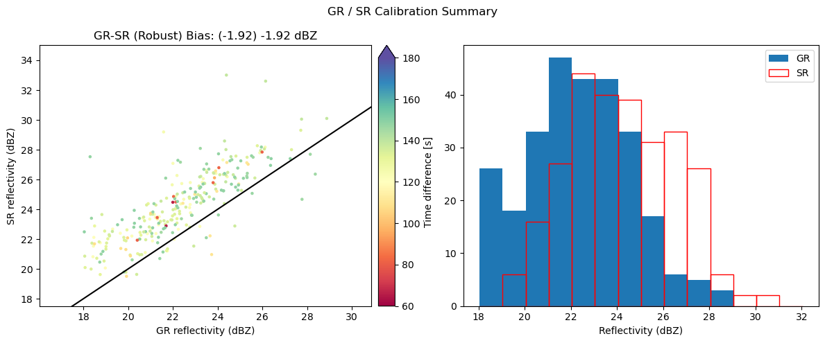
9. Determine GR calibration bias
The GR calibration bias can be obtained by averaging the difference between the matched SR/GR reflectivity measurements:
# Compute average offset
z_offset = np.nanmean(gdf_filtered[sr_z_column] - gdf_filtered[gr_z_column]).round(2)
z_offset_robust = np.nanmedian(gdf_filtered[sr_z_column] - gdf_filtered[gr_z_column]).round(2)

print(f"The ZH Calibration offset is (mean): {z_offset} dBZ")
print(f"The ZH Calibration offset is (median): {z_offset_robust} dBZ")
The ZH Calibration offset is (mean): 1.92 dBZ
The ZH Calibration offset is (median): 1.92 dBZ
Next steps
We encourage you to explore and adapt the code provided in this tutorial, analyze multiple GPM overpasses, and assess the long-term calibration bias of your ground radar network.
Please share any insights or suggestions for improving the matching procedure or filtering criteria with the GPM-API community so we can collaboratively enhance the routines.
We hope you enjoyed the tutorial! 😊
References
Citation
This notebook is part of the GPM-API documentation.
Copyright: GPM-API developers. Distributed under the MIT License. See GPM-API license for more info.
- Schwaller, M. R., & Morris, K. R. (2011). A Ground Validation Network for the Global Precipitation Measurement Mission. Journal of Atmospheric and Oceanic Technology, 28(3), 301–319. 10.1175/2010jtecha1403.1
- Warren, R. A., Protat, A., Siems, S. T., Ramsay, H. A., Louf, V., Manton, M. J., & Kane, T. A. (2018). Calibrating Ground-Based Radars against TRMM and GPM. Journal of Atmospheric and Oceanic Technology, 35(2), 323–346. 10.1175/jtech-d-17-0128.1
- Cao, Q., Hong, Y., Qi, Y., Wen, Y., Zhang, J., Gourley, J. J., & Liao, L. (2013). Empirical conversion of the vertical profile of reflectivity from Ku‐band to S‐band frequency. Journal of Geophysical Research: Atmospheres, 118(4), 1814–1825. 10.1002/jgrd.50138