Retrieving your first wind field#
3D variational technique#
PyDDA minimizes a cost function \(J\) that corresponds to various penalties including:
The cost function to be minimized is a weighted sum of the various cost functions in PyDDA and are represented in Equation (1):
\(J = c_{m}J_{m} + c_{o}J_{o} + c_{b}J_{b} + c_{s}J_{s} + ...\) (1)
Doing your first wind retrieval#
The next step is to use PyDDA to retrieve the input winds! In order to perform a wind retrieval, there are many aspects that must be considered. After the data processing has finished, it is now important to constrain the wind field further by adding in either sounding, point, or model data as a weak constraint in order to increase the chance that PyDDA will provide a solution that converges to a physically realistic wind field. For this particular example, we are lucky enough to have model data from the Rapid Update Cycle (RUC; the predecessor to the current Rapid Refresh/RAP) that can be used as a constraint.
Using PyDDA’s data model#
As of PyDDA 2.0, PyDDA uses xarray Datasets
to represent the underlying datastructure. This makes it easier to integrate PyDDA into xarray-based workflows
that are the standard for use in the Geoscientific Python Community. Therefore, anyone using PyART Grids will need
to convert their grids to PyDDA Grids using the pydda.io.read_from_pyart_grid() helper function.
grid_ktlx = pydda.io.read_from_pyart_grid(grid_ktlx)
grid_kict = pydda.io.read_from_pyart_grid(grid_kict)
In addition, pydda.io.read_grid() will read a cf-Compliant radar grid into a PyDDA Grid.
Using models for constraints#
In this example, we will use model data from the Rapid Update Cycle (RUC) in order to provide a constraint on the horizontal winds. This helps to constrain the background area where there is suboptimal coverage from the radar network outside of the dual Doppler lobes. To add either a RUC or HRRR model time period as a constraint, we need to have the original model data in GRIB format and then use the following line to load the model data into a PyDDA grid for processing.
# Add constraints
grid_kict = pydda.constraints.add_hrrr_constraint_to_grid(grid_kict,
    pydda.tests.get_sample_file('ruc2anl_130_20110520_0800_001.grb2'), method='linear')
Set up your initialization#
In addition to adding more constraints, PyDDA requires a first guess of the wind field in order to start performing the optimization loop that finds the wind field that minimizes \(J\). For this example, we will start with a zero initial wind field. The following code snippet will initialize PyDDA with a zero wind field:
grid_kict = pydda.initialization.make_constant_wind_field(grid_kict, (0.0, 0.0, 0.0))
Retrieving your first wind field#
We will then take a first attempt at retrieving a wind field using PyDDA. This is done using the
pydda.retrieval.get_dd_wind_field() function. This function takes in a minimum of one input, a list
of input PyART Grids. We will also specify the constants for the constraints. In this case, we are using
the mass continuity, radar observation, smoothness, and model constraints.
grids_out, _ = pydda.retrieval.get_dd_wind_field([grid_kict, grid_ktlx],
                                            Cm=256.0, Co=1e-2, Cx=1, Cy=1,
                                            Cz=1, Cmod=1e-5, model_fields=["hrrr"],
                                            refl_field='DBZ', wind_tol=0.5,
                                            max_iterations=50, filter_window=15,
                                            filter_order=3, engine='scipy')
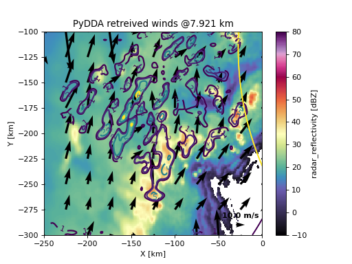
Plotting the output winds#
PyDDA contains visualization routines to create barb, quiver, and streamline plots of your wind fields
overlaid on gridded radar variables. Further detail about these visualization routines is contained in the
Visualizing the wind retrieval section. For this example, we will use pydda.vis.plot_horiz_xsection_quiver to
create a quiver plot of the wind field. In this example, we are plotting winds at the 15th vertical level of the
grid, with the background field being reflectivity with the colormap spanning -10 to 80 ref. We will specify 25 km
horizontal spacing between quivers and a quiver key length of 10 m/s. Finally, we specify that we will place the quiver
key on the bottom right interior of the plot.
pydda.vis.plot_horiz_xsection_quiver(grids_out, level=15, cmap='ChaseSpectral', vmin=-10, vmax=80,
                                 quiverkey_len=10.0, background_field='DBZ', bg_grid_no=1,
                                 w_vel_contours=[1, 2, 5, 10], quiver_spacing_x_km=25.0,
                                 quiver_spacing_y_km=25.0, quiverkey_loc='bottom_right')
(Source code, png, hires.png, pdf)

We can see in this figure that PyDDA is resolving numerous updrafts in the mid-levels. One thing to be aware of is the vertical motion at the edge of the Dual Doppler lobe in the top right corner. This vertical motion is likely caused by the wind source changing from primarily the radar data to the RUC model run outside of the Dual Doppler lobes, causing a slight shift in winds that results in horizontal convergence. This convergence will result in an updraft in the domain that is an artifact of this switch in data sources. It is therefore recommended to not use vertical velocity data in updrafts that are touching the Dual Doppler lobe edges to mitigate this issue. In addition, prescribing a stronger background constraint or filtering the data more often may also help mitigate this issue. We will go into this further in Optimizing your wind retrieval.