Radar Data Quality Control - Dealiasing#
In this notebook, we will showcase how to perform quality control of your radar files, specifically dealiasing velocities. By doing this we can provide PyDDA with quality controlled Doppler velocities for dual Doppler analysis.
Read the Data#
For this example, we use test data for two NEXRAD (WSR-88D) radars in northern Oklahoma: KTLX (Twin Lakes, OK) and KICT (Wichita, KS). For more information on reading the radar data, consult Reading in Radar Data in Native Radial Coordinates.
- Get test data::
https://arm-doe.github.io/pyart/API/generated/pyart.testing.get_test_data.html
- Reading CF-Radial::
https://arm-doe.github.io/pyart/API/generated/pyart.io.read_cfradial.html
# read in the data from both XSAPR radars
ktlx_file = pydda.tests.get_sample_file("cfrad.20110520_081431.542_to_20110520_081813.238_KTLX_SUR.nc")
kict_file = pydda.tests.get_sample_file("cfrad.20110520_081444.871_to_20110520_081914.520_KICT_SUR.nc")
radar_ktlx = pyart.io.read_cfradial(ktlx_file)
radar_kict = pyart.io.read_cfradial(kict_file)
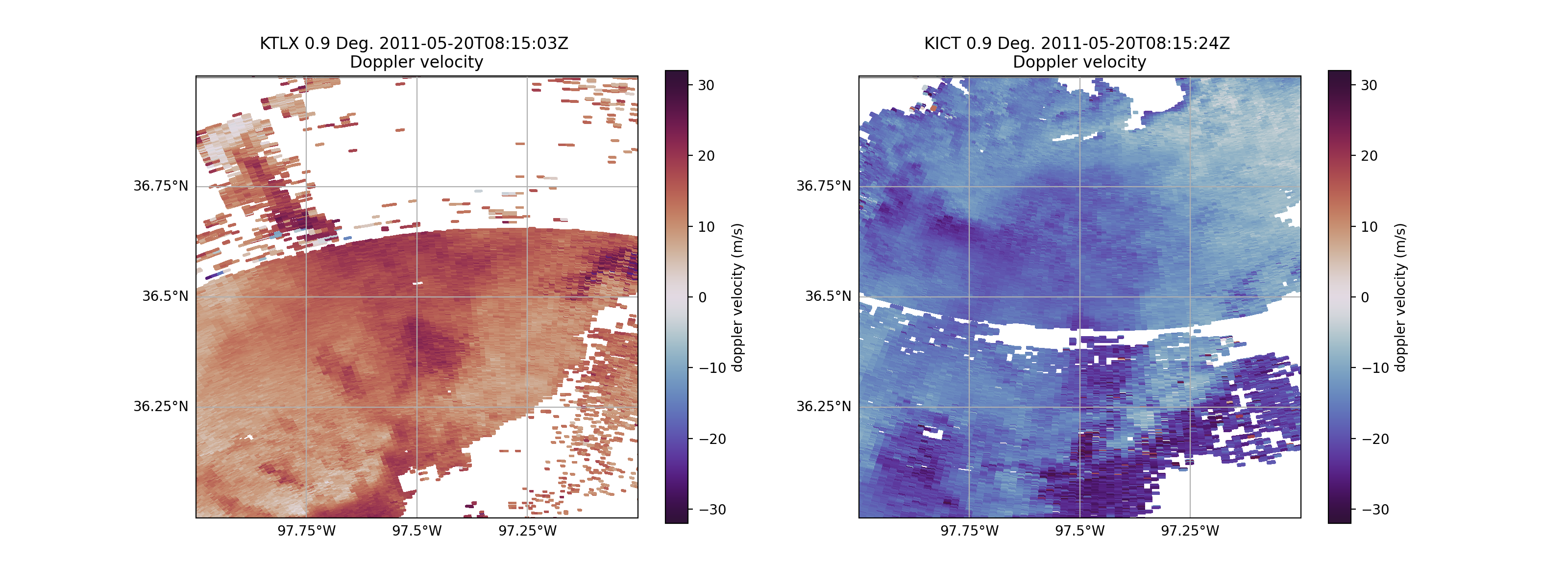
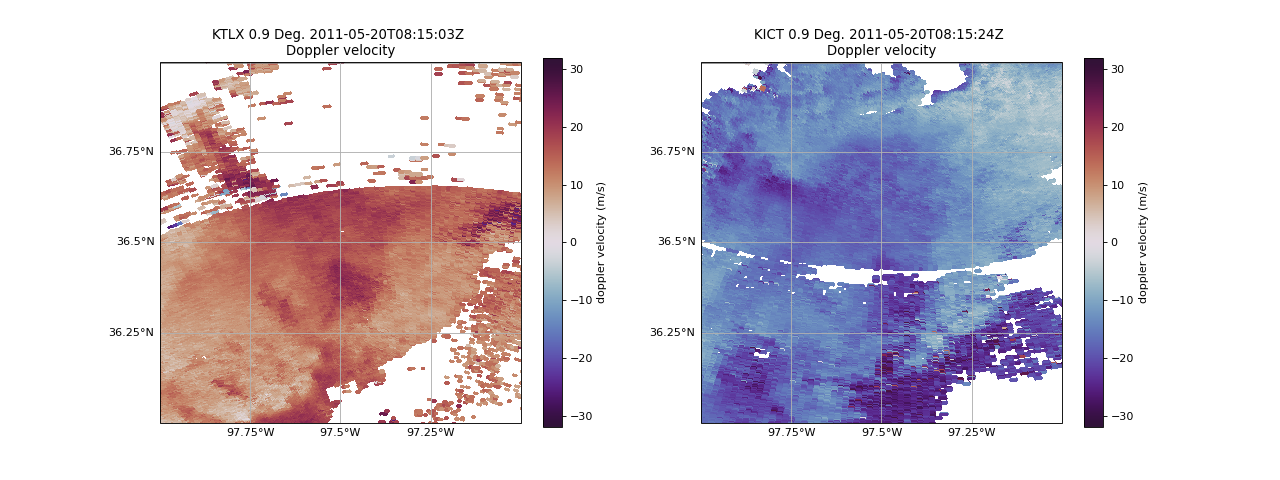
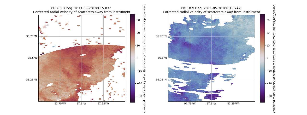
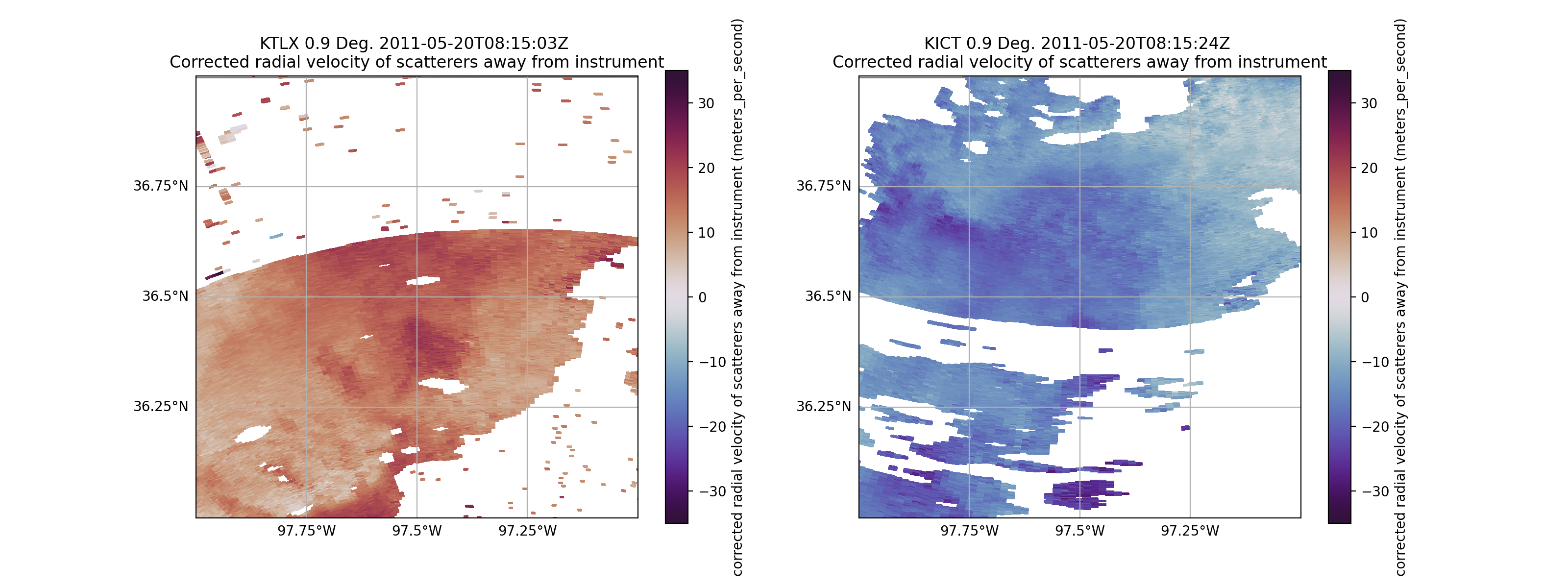
Plot Velocity of Both Radars#
fig = plt.figure(figsize=(16, 6))
ax = plt.subplot(121, projection=ccrs.PlateCarree())

# Plot the southwestern radar
disp1 = pyart.graph.RadarMapDisplay(radar_ktlx)
disp1.plot_ppi_map(
    "VEL",
    sweep=1,
    ax=ax,
    vmin=-32,
    vmax=32,
    min_lat=36,
    max_lat=37,
    min_lon=-98,
    max_lon=-97,
    lat_lines=np.arange(36, 37.25, 0.25),
    lon_lines=np.arange(-98, -96.75, 0.25),
    cmap='twilight_shifted'
)

# Plot the southeastern radar
ax2 = plt.subplot(122, projection=ccrs.PlateCarree())
disp2 = pyart.graph.RadarMapDisplay(radar_kict)
disp2.plot_ppi_map(
    "VEL",
    sweep=1,
    ax=ax2,
    vmin=-32,
    vmax=32,
    min_lat=36,
    max_lat=37,
    min_lon=-98,
    max_lon=-97,
    lat_lines=np.arange(36, 37.25, 0.25),
    lon_lines=np.arange(-98, -96.75, 0.25),
    cmap='twilight_shifted'
)
(Source code, png, hires.png, pdf)
Determining Artifacts within Doppler Velocities#
Before dealiasing the radar velocities, we need to remove noise and clutter from the radar objects. Utilizing Py-ART, we will accomplish this by calculating the velocity texture, or the standard deviation of velocity surrounding a gate.
- Py-ART’s calculate_velocity_texture function::
https://arm-doe.github.io/pyart/API/generated/pyart.retrieve.calculate_velocity_texture.html
# Calculate the Velocity Texture and apply the PyART GateFilter Utility
vel_tex_ktlx = pyart.retrieve.calculate_velocity_texture(radar_ktlx,
                                                       vel_field='VEL',
                                                       )
vel_tex_kict = pyart.retrieve.calculate_velocity_texture(radar_kict,
                                                       vel_field='VEL',
                                                       )

## Add velocity texture to the radar objects
radar_ktlx.add_field('velocity_texture', vel_tex_ktlx, replace_existing=True)
radar_kict.add_field('velocity_texture', vel_tex_kict, replace_existing=True)
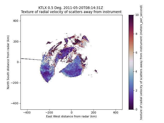
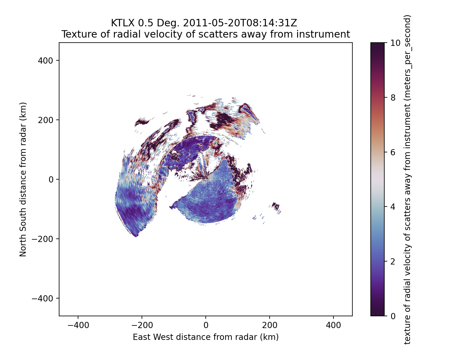
Velocity Texture Displays#
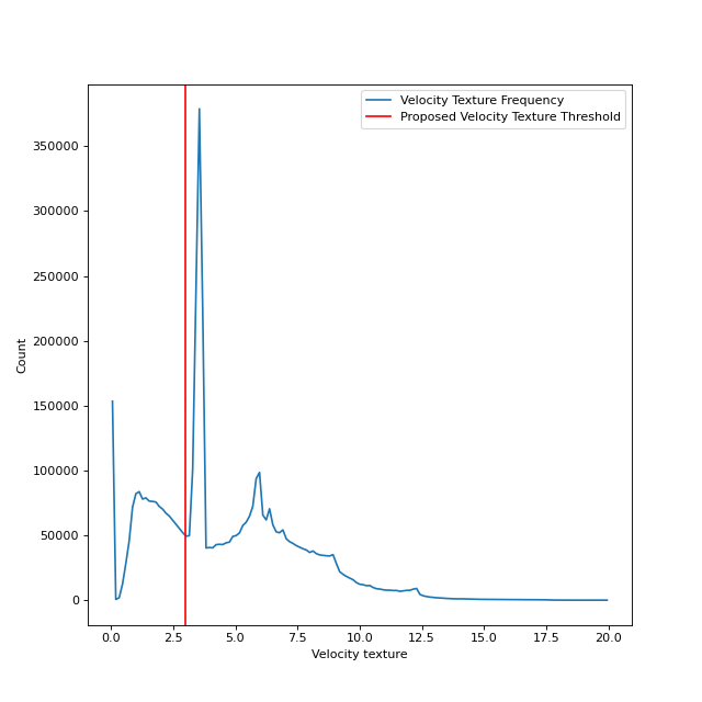
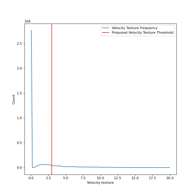
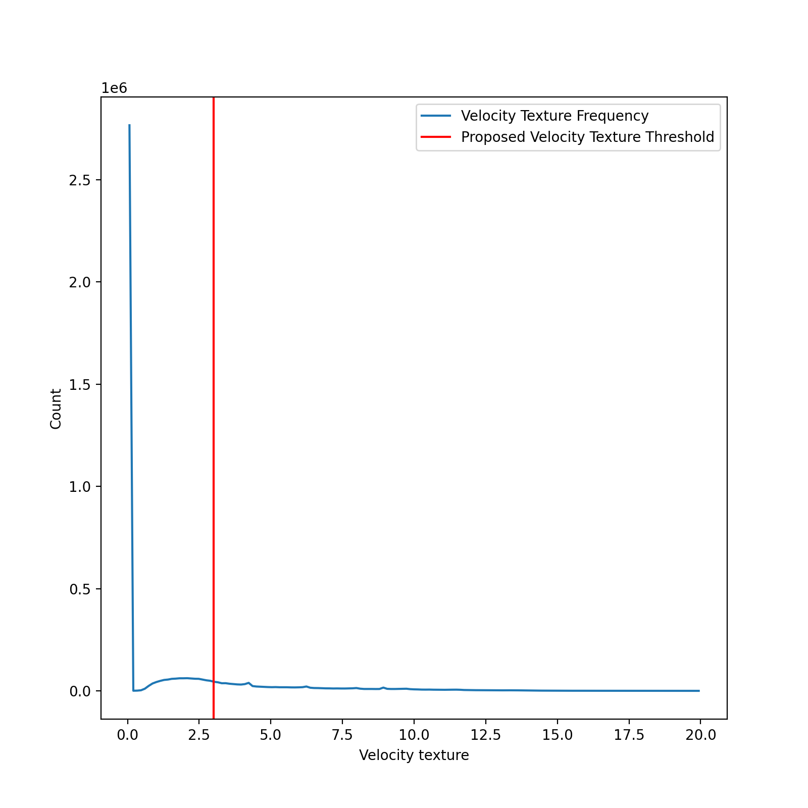
Let’s see what this velocity texture looks like. Additionally, a histogram of velocity texture values will allow for the determination of a threshold to distinguish the hydrometeor signal from artifacts.
# Display the calculated velocity texture
fig = plt.figure(figsize=[8, 6])
display = pyart.graph.RadarDisplay(radar_ktlx)
display.plot_ppi('velocity_texture',
                     sweep=0,
                     vmin=0,
                     vmax=10,
                     cmap=plt.get_cmap('twilight_shifted')
                     )

# Plot a histogram of the velocity textures
fig = plt.figure(figsize=[8, 8])
hist, bins = np.histogram(radar_ktlx.fields['velocity_texture']['data'],
                          bins=np.linspace(0, 20, 150))
bins = (bins[1:]+bins[:-1])/2.0
plt.plot(bins,
         hist,
         label='Velocity Texture Frequency'
         )
plt.axvline(3,
            color='r',
            label='Proposed Velocity Texture Threshold'
            )
plt.xlabel('Velocity texture')
plt.ylabel('Count')
plt.legend()
Filter Doppler Velocity Artifacts#
Now that we have determined which velocity texture values correspond to artifacts within the Doppler velocity data, we utilize Py-ART’s GateFilter to filter out these artifacts
- Py-ART’s GateFilter function::
https://arm-doe.github.io/pyart/API/generated/pyart.filters.GateFilter.html
# Apply a GateFilter
gatefilter_ktlx = pyart.filters.GateFilter(radar_ktlx)
gatefilter_ktlx.exclude_above('velocity_texture', 3)
gatefilter_kict = pyart.filters.GateFilter(radar_kict)
gatefilter_kict.exclude_above('velocity_texture', 3)
Apply Dealiasing#
Now that we have removed artifacts, we can proceed with dealiasing the Doppler velocity data with Py-ART’s Region-Based Dealiasing Algorithm.
The Region-Based Dealiasing finds regions of similar velocities and unfolds and merges these pairs of regions until all data are unfolded.
- Py-ART’s Region Based Dealiasing Correction::
https://arm-doe.github.io/pyart/API/generated/pyart.correct.dealias_region_based.html
# Apply Region Based DeAlising Utiltiy
vel_dealias_ktlx = pyart.correct.dealias_region_based(radar_ktlx,
                                                    vel_field='VEL',
                                                    centered=True,
                                                    gatefilter=gatefilter_ktlx
                                                    )

# Apply Region Based DeAlising Utiltiy
vel_dealias_kict = pyart.correct.dealias_region_based(radar_kict,
                                                    vel_field='VEL',
                                                    centered=True,
                                                    gatefilter=gatefilter_kict
                                                    )

# Add our data dictionary to the radar object
radar_kict.add_field('corrected_velocity', vel_dealias_kict, replace_existing=True)
radar_ktlx.add_field('corrected_velocity', vel_dealias_ktlx, replace_existing=True)
Display Corrected Velocity Fields#
Let’s check on our corrected velocity fields!
fig = plt.figure(figsize=(16, 6))

# Plot the southwestern radar
ax = plt.subplot(121, projection=ccrs.PlateCarree())
disp1 = pyart.graph.RadarMapDisplay(radar_ktlx)
disp1.plot_ppi_map("corrected_velocity",
                   sweep=1,
                   ax=ax,
                   vmin=-35,
                   vmax=35,
                   min_lat=36,
                   max_lat=37,
                   min_lon=-98,
                   max_lon=-97,
                   lat_lines=np.arange(36, 37.25, 0.25),
                   lon_lines=np.arange(-98, -96.75, 0.25),
                   cmap=plt.get_cmap('twilight_shifted')
)

# Plot the southeastern radar
ax2 = plt.subplot(122, projection=ccrs.PlateCarree())
disp2 = pyart.graph.RadarMapDisplay(radar_kict)
disp2.plot_ppi_map("corrected_velocity",
                   sweep=1,
                   ax=ax2,
                   vmin=-35,
                   vmax=35,
                   min_lat=36,
                   max_lat=37,
                   min_lon=-98,
                   max_lon=-97,
                   lat_lines=np.arange(36, 37.25, 0.25),
                   lon_lines=np.arange(-98, -96.75, 0.25),
                   cmap=plt.get_cmap('twilight_shifted')
)
(Source code, png, hires.png, pdf)
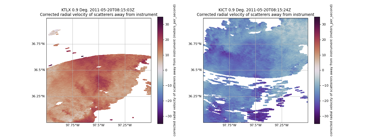
Summary#
Utilizing Py-ART, we read in two radar files within close proximity to each other. We then corrected the radar Doppler velocities to remove artifacts and clutter. Finally, utilizing Py-ART, we applied a region-based dealiasing algorithm to unfold the Doppler velocities.
Now that we have corrected velocities, incorporating these radars into PyDDA will be shown in the next notebook.