Converting the radar data to Cartesian coordinates with Py-ART#
PyDDA expects radar data to be in Cartesian coordinates before it retrieves the wind fields. Most radar data, however, is in the radar’s native antenna coordinates. Therefore, the radar data needs to be converted to Cartesian coordinates. Py-ART’s mapping toolbox contains the necessary utilities
We will assume that you have followed the steps outlined in Reading in Radar Data in Native Radial Coordinates for reading the radar data in its native coordinates. PyDDA requires dealiased velocities with noise, ground clutter, and second trip echoes removed for proper wind retrieval. Therefore, make sure you have first followed the instructions in Radar Data Quality Control - Dealiasing to correct the Doppler velocity data.
Gridding the data#
After the Doppler velocity data is corrected, it needs to be projected from the radar’s native antenna coordinates to Cartesian coordinates.
First, we need to determine a grid spacing that we want to use for the coordinate system. The X-band radars have a maximum unambiguous range of 50 km, so we do want to expand our grid to include areas 50 km away fron one of the radars
In addition, we want to be careful with our choice of grid resolution. For example, if we choose too fine of a grid resolution, then there may not be enough radar coverage available for making the input radial velocity fields continuous. This can cause your retrieval to have artificial noise, especially in updraft velocity. Therefore, you will need to choose a grid spacing that is coarse enough to have a continuous input radial velocity field at all altitudes. For example, Kosiba et al. (2013) chose their grid spacing such that it is about 1/2.5 the data spacing at the feature of interest. In this example, we will elect for a 500 m grid spacing. In addition, for the interest of having a wind retrieval done in a reasonable time frame for this example, we will limit the domain to the updrafts of interest.
grid_limits = ((0., 15000.), (-50000., 50000.), (-50000., 50000.))
grid_shape = (31, 201, 201)
The grid_limits is a 3-tuple of 2-tuples specifying the \(z\), \(y\), and \(x\)
limits of the grid in meters. The grid_shape specifies the shape of the grid in number of
points. We then use PyART’s grid_from_radars
function to create the grids grid_ktlx and grid_kict. PyDDA requires that both grids have the same
shape and origin, so we explicitly set those in the options for both grids.
grid_ktlx = pyart.map.grid_from_radars([radar_ktlx], grid_limits=grid_limits,
                                grid_shape=grid_shape, gatefilter=gatefilter_ktlx,
                                grid_origin=(radar_kict.latitude['data'].filled(),
                                             radar_kict.longitude['data'].filled()))
grid_kict = pyart.map.grid_from_radars([radar_kict], grid_limits=grid_limits,
                                grid_shape=grid_shape, gatefilter=gatefilter_kict,
                                grid_origin=(radar_kict.latitude['data'].filled(),
                                             radar_kict.longitude['data'].filled()))
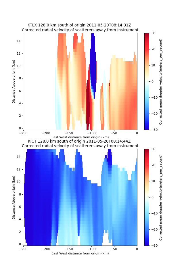
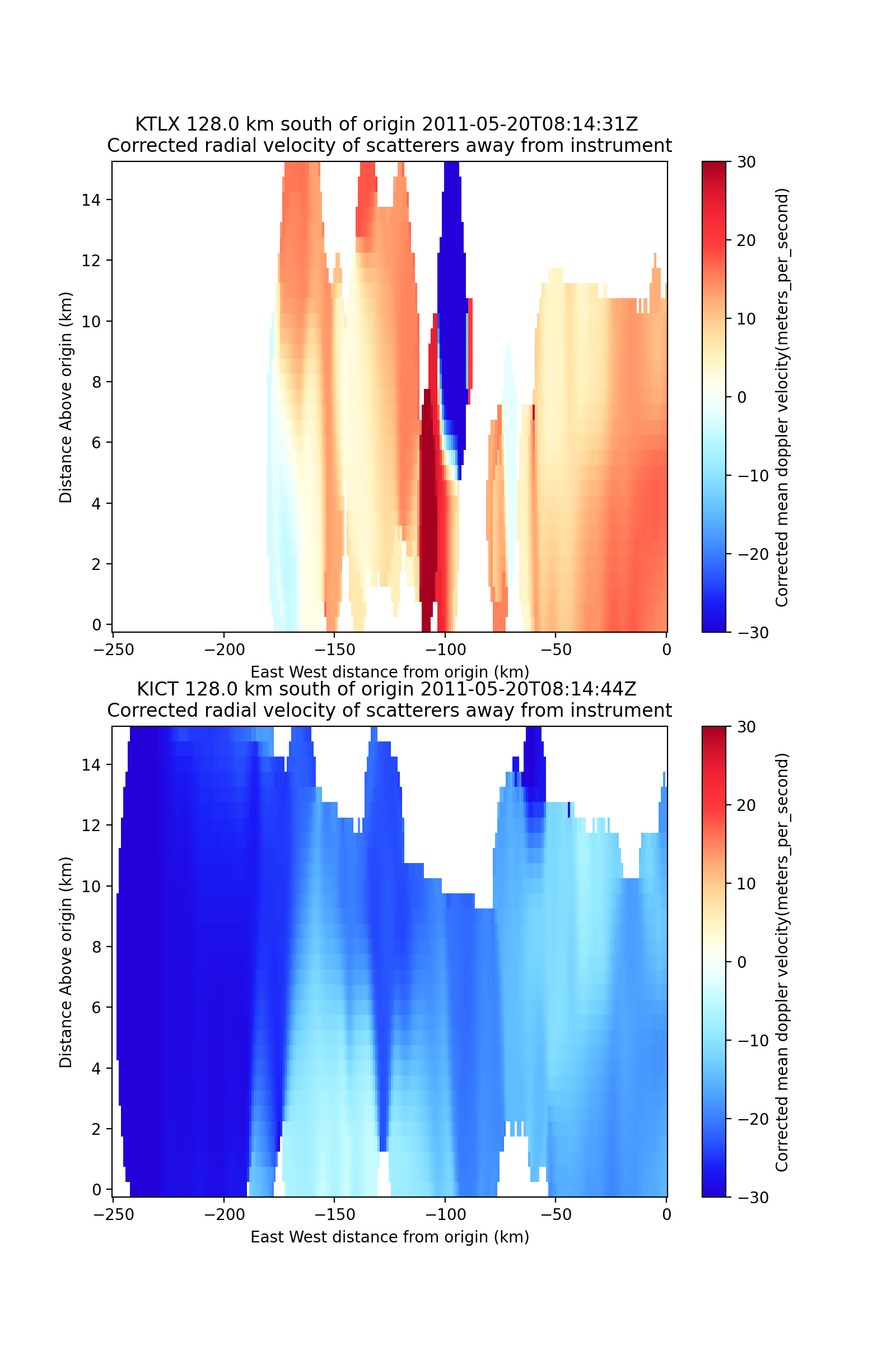
Finally, we should visualize the output grids using Py-ART’s GridMapDisplay.
fig = plt.figure(figsize=(8, 12))
ax1 = plt.subplot(211)
display1 = pyart.graph.GridMapDisplay(grid_ktlx)
display1.plot_latitude_slice('corrected_velocity', lat=36.5,
                             ax=ax1, fig=fig, vmin=-30, vmax=30)
ax2 = plt.subplot(212)
display2 = pyart.graph.GridMapDisplay(grid_kict)
display2.plot_latitude_slice('corrected_velocity', lat=36.5,
                             ax=ax2, fig=fig, vmin=-30, vmax=30)
(Source code, png, hires.png, pdf)
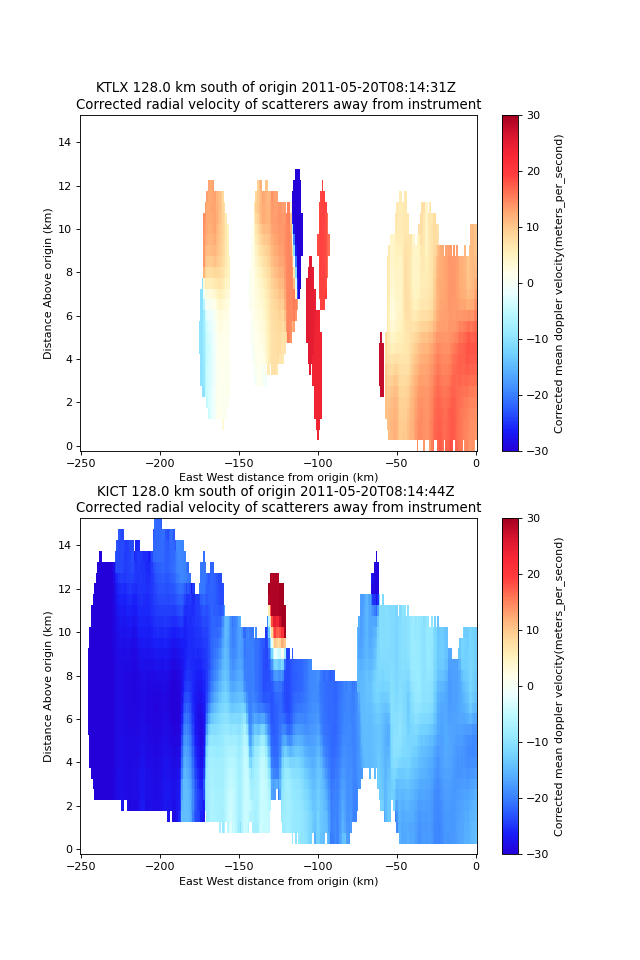
Note that, as the spacing between the sweeps increases with altitude that there can be gridding artifacts that can produce spurious air motion in the retrievals (Collis et al. 2010). To reduce these artifacts it’s important that the velocity field at higher altitudes be as continuous as possible. This requires a grid resolution that will you will need to balance with keeping important details of the feature of interest that you are trying to grid. You may have to adjust your grid resolution to balance these two concerns in order to properly retrieve wind velocities. With the current grid spacing, it is apparent that there are discontinuities in the radial velocity field above 7.5 km altitude that could cause spurious noise in the retrieved vertical velocity field. Vertical velocities are likely to be most reliable about 20-40 km from either radar.
References#
Collis, S., A. Protat, and K. Chung, 2010: The Effect of Radial Velocity Gridding Artifacts on Variationally Retrieved Vertical Velocities. J. Atmos. Oceanic Technol., 27, 1239–1246, https://doi.org/10.1175/2010JTECHA1402.1.
Koch, S. E., M. desJardins, and P. J. Kocin, 1983: An Interactive Barnes Objective Map Analysis Scheme for Use with Satellite and Conventional Data. J. Appl. Meteor. Climatol., 22, 1487–1503, https://doi.org/10.1175/1520-0450(1983)022<1487:AIBOMA>2.0.CO;2.
Kosiba, K., J. Wurman, Y. Richardson, P. Markowski, P. Robinson, and J. Marquis, 2013: Genesis of the Goshen County, Wyoming, Tornado on 5 June 2009 during VORTEX2. Mon. Wea. Rev., 141, 1157–1181, https://doi.org/10.1175/MWR-D-12-00056.1.