In this tutorial, we will provide the foundations to use GPM-API to download, manipulate and analyze data from the Global Precipitation Measurement (GPM) spaceborne radars.
Please note that GPM-API also enable access and analysis tools for the entire GPM constellation of passive microwave sensors as well as the IMERG precipitation products. For detailed information and additional tutorials, please refer to the official GPM-API documentation.
First, let’s import the package required in this tutorial.
import datetime
import gpm
import fsspec
import numpy as np
import ximage  # noqa
import xarray as xr
from xarray.backends.api import open_datatree
import matplotlib.pyplot as plt
import cartopy.crs as ccrs
from gpm.utils.geospatial import (
    get_country_extent,
    get_geographic_extent_around_point,
    get_circle_coordinates_around_point,
)
from gpm.gv import volume_matching, compare_maps, calibration_summary
Using the available_products function, users can obtain a list of all GPM products that can be downloaded and opened into CF-compliant xarray datasets.
gpm.available_products(product_types="RS") # research products['1A-GMI',
'1A-TMI',
'1B-GMI',
'1B-Ka',
'1B-Ku',
'1B-PR',
'1B-TMI',
'1C-AMSR2-GCOMW1',
'1C-AMSRE-AQUA',
'1C-AMSUB-NOAA15',
'1C-AMSUB-NOAA16',
'1C-AMSUB-NOAA17',
'1C-ATMS-NOAA20',
'1C-ATMS-NOAA21',
'1C-ATMS-NPP',
'1C-GMI',
'1C-GMI-R',
'1C-MHS-METOPA',
'1C-MHS-METOPB',
'1C-MHS-METOPC',
'1C-MHS-NOAA18',
'1C-MHS-NOAA19',
'1C-SAPHIR-MT1',
'1C-SSMI-F08',
'1C-SSMI-F10',
'1C-SSMI-F11',
'1C-SSMI-F13',
'1C-SSMI-F14',
'1C-SSMI-F15',
'1C-SSMIS-F16',
'1C-SSMIS-F17',
'1C-SSMIS-F18',
'1C-SSMIS-F19',
'1C-TMI',
'2A-AMSR2-GCOMW1',
'2A-AMSR2-GCOMW1-CLIM',
'2A-AMSRE-AQUA-CLIM',
'2A-AMSUB-NOAA15-CLIM',
'2A-AMSUB-NOAA16-CLIM',
'2A-AMSUB-NOAA17-CLIM',
'2A-ATMS-NOAA20',
'2A-ATMS-NOAA20-CLIM',
'2A-ATMS-NOAA21',
'2A-ATMS-NOAA21-CLIM',
'2A-ATMS-NPP',
'2A-ATMS-NPP-CLIM',
'2A-DPR',
'2A-ENV-DPR',
'2A-ENV-Ka',
'2A-ENV-Ku',
'2A-ENV-PR',
'2A-GMI',
'2A-GMI-CLIM',
'2A-GPM-SLH',
'2A-Ka',
'2A-Ku',
'2A-MHS-METOPA',
'2A-MHS-METOPA-CLIM',
'2A-MHS-METOPB',
'2A-MHS-METOPB-CLIM',
'2A-MHS-METOPC',
'2A-MHS-METOPC-CLIM',
'2A-MHS-NOAA18',
'2A-MHS-NOAA18-CLIM',
'2A-MHS-NOAA19',
'2A-MHS-NOAA19-CLIM',
'2A-PR',
'2A-SAPHIR-MT1',
'2A-SAPHIR-MT1-CLIM',
'2A-SSMI-F08-CLIM',
'2A-SSMI-F10-CLIM',
'2A-SSMI-F11-CLIM',
'2A-SSMI-F13-CLIM',
'2A-SSMI-F14-CLIM',
'2A-SSMI-F15-CLIM',
'2A-SSMIS-F16',
'2A-SSMIS-F16-CLIM',
'2A-SSMIS-F17',
'2A-SSMIS-F17-CLIM',
'2A-SSMIS-F18',
'2A-SSMIS-F18-CLIM',
'2A-SSMIS-F19',
'2A-SSMIS-F19-CLIM',
'2A-TMI-CLIM',
'2A-TRMM-SLH',
'2B-GPM-CORRA',
'2B-GPM-CSAT',
'2B-GPM-CSH',
'2B-TRMM-CORRA',
'2B-TRMM-CSAT',
'2B-TRMM-CSH',
'IMERG-FR']Let’s have a look at the available RADAR products:
gpm.available_products(product_categories="RADAR", product_levels="1B")['1B-Ka', '1B-Ku', '1B-PR']gpm.available_products(product_categories="RADAR", product_levels="2A")['2A-DPR',
'2A-ENV-DPR',
'2A-ENV-Ka',
'2A-ENV-Ku',
'2A-ENV-PR',
'2A-GPM-SLH',
'2A-Ka',
'2A-Ku',
'2A-PR',
'2A-TRMM-SLH']In this tutorial, we will use the 2A-DPR product which provides the GPM Dual-frequency Precipitation Radar (DPR) reflectivities and associated precipitation retrievals.
Since we are running this tutorial on a Binder environment, we will not execute the following gpm.download and gpm.open_dataset sections, and directly load the 2A.GPM.DPR.V9-20211125.20230820-S213941-E231213.053847.V07B.HDF5 granule file,
which has been preconverted to a Zarr Store and uploaded on the Pythia Cloud Bucket to simplify access to the data.
1. Download Data
Now let’s download the 2A-DPR product over a couple of hours.
To download GPM data with GPM-API, you have to previously create a NASA Earthdata and/or NASA PPS account. We provide a step-by-step guide on how to set up your accounts in the official GPM-API documentation.
# Specify the time period you are interested in
start_time = datetime.datetime.strptime("2023-08-20 22:12:00", "%Y-%m-%d %H:%M:%S")
end_time = datetime.datetime.strptime("2023-08-20 22:13:45", "%Y-%m-%d %H:%M:%S")
# Specify the product and product type
product = "2A-DPR"  # 2A-PR
product_type = "RS"
storage = "GES_DISC"
# Specify the version
version = 7
# Download the data
# gpm.download(
# product=product,
# product_type=product_type,
# version=version,
# start_time=start_time,
# end_time=end_time,
# storage=storage,
# force_download=False,
# verbose=True,
# progress_bar=True,
# check_integrity=False,
# )Once, the data are downloaded on disk, let’s load the 2A-DPR product and look at the dataset structure.
2. Load Data
With GPM-API, the name granule is used to refer to a single file, while the name dataset is used to refer to a collection of granules.
GPM-API enables to open single or multiple granules into an xarray.Dataset, an object designed for working with labeled multi-dimensional arrays.
The
gpm.open_granule(filepath)opens a single file into xarray by providing the path of the file of interest.The
gpm.open_datasetfunction enables to open a collection of granules over a period of interest.
# Load the 2A-DPR dataset

# ds = gpm.open_dataset(
#     product=product,
#     product_type=product_type,
#     version=version,
#     start_time=start_time,
#     end_time=end_time,
# )
# ds
Here we directly read the data required for this tutorial from the Pythia Cloud Bucket so that you don’t have to register a NASA account and download the data beforehand.
bucket_url = "https://js2.jetstream-cloud.org:8001"
fs = fsspec.filesystem("s3", anon=True, client_kwargs=dict(endpoint_url=bucket_url))
file = fs.get_mapper(
    f"pythia/radar/erad2024/gpm_api/2A.GPM.DPR.V9-20211125.20230820-S213941-E231213.053847.V07B.zarr"
)
ds = xr.open_zarr(file, consolidated=True, chunks={})
3. Basic Manipulations
You can list variables, coordinates and dimensions with the following methods:
# Available variables
print("Available variables: ", list(ds.data_vars))
# Available coordinates
print("Available coordinates: ", list(ds.coords))
# Available dimensions
print("Available dimensions: ", list(ds.dims))
# Spatial dimension:
print("Spatial dimensions: ", ds.gpm.spatial_dimensions)
# Vertical dimension:
print("Vertical dimension: ", ds.gpm.vertical_dimension)
Available variables: ['DFRforward1', 'Dm', 'FractionalGranuleNumber', 'MSindex', 'MSindexKa', 'MSindexKu', 'MSkneeDFRindex', 'MSslopesKa', 'MSslopesKu', 'MSsurfPeakIndexKa', 'MSsurfPeakIndexKu', 'NUBFindex', 'Nw', 'PIAalt', 'PIAdw', 'PIAhb', 'PIAhybrid', 'PIAweight', 'PIAweightHY', 'RFactorAlt', 'acsModeMidScan', 'adjustFactor', 'airTemperature', 'alongTrackBeamWidth', 'attenuationNP', 'binBBBottom', 'binBBPeak', 'binBBTop', 'binClutterFreeBottom', 'binDFRmMLBottom', 'binDFRmMLTop', 'binEchoBottom', 'binHeavyIcePrecipBottom', 'binHeavyIcePrecipTop', 'binMirrorImageL2', 'binMixedPhaseTop', 'binNode', 'binRealSurface', 'binStormTop', 'binZeroDeg', 'binZeroDegSecondary', 'crossTrackBeamWidth', 'dBNw', 'dataWarning', 'dprAlt', 'echoCountRealSurface', 'elevation', 'ellipsoidBinOffset', 'epsilon', 'flagAnvil', 'flagBB', 'flagEcho', 'flagGraupelHail', 'flagHail', 'flagHeavyIcePrecip', 'flagInversion', 'flagMLquality', 'flagPrecip', 'flagSLV', 'flagScanPattern', 'flagSensor', 'flagShallowRain', 'flagSigmaZeroSaturation', 'flagSurfaceSnowfall', 'geoError', 'geoWarning', 'greenHourAng', 'heightBB', 'heightStormTop', 'heightZeroDeg', 'landSurfaceType', 'limitErrorFlag', 'localZenithAngle', 'missing', 'modeStatus', 'nHeavyIcePrecip', 'operationalMode', 'paramNUBF', 'paramRDm', 'pathAtten', 'phase', 'phaseNearSurface', 'piaExp', 'piaFinal', 'piaNP', 'piaNPrainFree', 'piaOffset', 'pointingStatus', 'precipRate', 'precipRateAve24', 'precipRateESurface', 'precipRateESurface2', 'precipRateESurface2Status', 'precipRateNearSurface', 'precipWater', 'precipWaterIntegrated', 'precipWaterIntegrated_Liquid', 'precipWaterIntegrated_Solid', 'qualityBB', 'qualityData', 'qualityFlag', 'qualitySLV', 'qualityTypePrecip', 'range_distance_from_satellite', 'refScanID', 'reliabFactor', 'reliabFactorHY', 'reliabFlag', 'reliabFlagHY', 'scAlt', 'scAttPitchGeoc', 'scAttPitchGeod', 'scAttRollGeoc', 'scAttRollGeod', 'scAttYawGeoc', 'scAttYawGeod', 'scHeadingGround', 'scHeadingOrbital', 'scLat', 'scLon', 'scPos', 'scVel', 'seaIceConcentration', 'sigmaZeroCorrected', 'sigmaZeroMeasured', 'sigmaZeroNPCorrected', 'sigmaZeroProfile', 'snRatioAtRealSurface', 'snowIceCover', 'stddevEff', 'stddevHY', 'surfaceSnowfallIndex', 'targetSelectionMidScan', 'timeMidScan', 'timeMidScanOffset', 'typePrecip', 'widthBB', 'zFactorFinal', 'zFactorFinalESurface', 'zFactorFinalNearSurface', 'zFactorMeasured', 'zeta']
Available coordinates: ['DSD_params', 'SCorientation', 'crsWGS84', 'dataQuality', 'gpm_along_track_id', 'gpm_cross_track_id', 'gpm_granule_id', 'gpm_id', 'gpm_range_id', 'height', 'lat', 'lon', 'radar_frequency', 'range', 'sunLocalTime', 'time']
Available dimensions: ['cross_track', 'along_track', 'range', 'DSD_params', 'four', 'method', 'radar_frequency', 'three', 'nfreqHI', 'nNode', 'nNUBF', 'nNP', 'foreBack', 'nearFar', 'XYZ', 'nbinSZP', 'nsdew']
Spatial dimensions: ['along_track', 'cross_track']
Vertical dimension: ['range']
Through the use of the xarray gpm accessor, you can access various methods that simplify for example the listing of variables according to their dimensions.
For example, using ds.gpm.spatial_3d_variables you can list all dataset variables with spatial horizontal and vertical dimensions, while with
ds.gpm.spatial_2d_variables you can list all dataset variables with only spatial horizontal dimensions.
To directly obtain a dataset with the variables of interest, you can also call the ds.gpm.select_spatial_2d_variables or ds.gpm.select_spatial_3d_variables methods.
Please keep in mind that to create a spatial map, it is necessary to select spatial 2D variables, while for extracting vertical cross-sections it is necessary to slice across spatial 3D variables.
print(ds.gpm.spatial_2d_variables)
ds.gpm.select_spatial_2d_variables()print(ds.gpm.spatial_3d_variables)
ds.gpm.select_spatial_3d_variables()Some variables also have a frequency dimension. You can list or subset such variables using ds.gpm.frequency_variables and ds.gpm.'select_frequency_variables respectively.
print(ds.gpm.frequency_variables)
ds.gpm.select_frequency_variables()Using the ds.gpm.bin_variables or ds.gpm.select_bin_variables you can instead list or select the variables that contains “pointers” to specific radar gates.
The bin variables are useful to slice or extract data across the “range” dimension of the dataset.
Bin variables values range from 1 (the ellipsoid surface) to the size of the range dimension (in the upper atmosphere).
print(ds.gpm.bin_variables)
ds.gpm.select_bin_variables()To select the DataArray corresponding to a single variable you do:
variable = "precipRateNearSurface"
da = ds[variable]
print(" Array Class: ", type(da.data))
daIf the array class is dask.Array, it means that the data are not yet loaded into RAM memory.
To put the data into memory, you need to call the method compute, either on the xarray object or on the numerical array.
da = da.compute()
print("Array Class: ", type(da.data))
daTo check if the Dataset or the DataArray you selected has only spatial horizontal and/or vertical dimensions, you can use the xarray accessor gpm.is_spatial_2d and gpm.is_spatial_3d properties.
print(
    ds.gpm.is_spatial_2d
)  # False because the xarray.Dataset also contains the range and frequency dimensions !
print(
    ds.gpm.is_spatial_3d
)  # False because the xarray.Dataset also contains frequency dimensions !
False
False
print(
    ds["zFactorFinal"].isel(range=0).sel(radar_frequency="Ka").gpm.is_spatial_2d
)  # True
print(ds["precipRateNearSurface"].gpm.is_spatial_2d)
True
True
You can select the reflectivity volumes at a given frequency using the radar band name with the sel method:
ds["zFactorFinal"].sel(radar_frequency="Ka")Since xarray does not yet allow subsetting by value along non-dimensional coordinates, the gpm.sel method provides you this functionality.
As an example, you can subset the dataset by time:
start_time = datetime.datetime.strptime("2023-08-20 22:12:00", "%Y-%m-%d %H:%M:%S")
end_time = datetime.datetime.strptime("2023-08-20 22:13:45", "%Y-%m-%d %H:%M:%S")
ds_subset = ds.gpm.sel(time=slice(start_time, end_time))
ds_subset["time"]Remember that you can get the start time and end time of your GPM xarray object with the gpm accessor methods start_time and end_time.
print(ds_subset.gpm.start_time)
print(ds_subset.gpm.end_time)
2023-08-20 22:12:00
2023-08-20 22:13:45
You can also subset your GPM xarray object by gpm_id, gpm_cross_track_id or gpm_range_id coordinates, which act as reference identifiers for the along-track, cross-track and range dimensions.
Selecting across coordinates by value is useful for example to:
- align multiple GPM xarray objects that might have been subsetted differently across the
cross_track,along_trackorrangedimensions. - to retrieve a specific portion of a GPM granule indipendently of the previous subsetting operations.
The gpm_id is defined as <gpm_granule_number>-<gpm_along_track_id>, while the others <gpm_*_id> coordinates start at 0 and increase incrementally by 1 along each granule dimension.
# Subset by gpm_id
start_gpm_id = "53847-2768"
end_gpm_id = "53847-2918"
ds_subset = ds.gpm.sel(gpm_id=slice(start_gpm_id, end_gpm_id))
ds_subset["gpm_id"].dataTo check whether the GPM 2A-DPR product has contiguous along-track scans (with no missing scans), you can use:
print(ds.gpm.has_contiguous_scans)
print(ds.gpm.is_regular)
True
True
In case there are non-contiguous scans, you can obtain the along-track slices over which the dataset is regular:
list_slices = ds.gpm.get_slices_contiguous_scans()
print(list_slices)
[slice(0, 7932, None)]
You can then select a regular portion of the dataset with:
slc = list_slices[0]
print(slc)
ds_regular = ds.isel(along_track=slc)
slice(0, 7932, None)
4. Plot Maps
The GPM-API provides two ways of displaying 2D spatial fields:
- The
plot_mapmethod plot the data in a geographic projection using the Cartopypcolormeshmethod. - The
plot_imagemethod plot the data as an image using the xarrayimshowmethod.
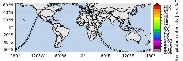
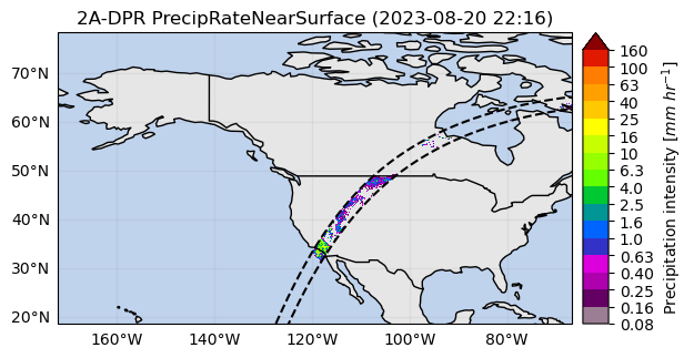
Let’s start by plotting the entire GPM DPR granule in the geographic space:
ds[variable].gpm.plot_map()<cartopy.mpl.geocollection.GeoQuadMesh at 0x7f66f403efd0>/srv/conda/envs/notebook/lib/python3.11/site-packages/cartopy/io/__init__.py:241: DownloadWarning: Downloading: https://naturalearth.s3.amazonaws.com/110m_physical/ne_110m_land.zip
warnings.warn(f'Downloading: {url}', DownloadWarning)
/srv/conda/envs/notebook/lib/python3.11/site-packages/cartopy/io/__init__.py:241: DownloadWarning: Downloading: https://naturalearth.s3.amazonaws.com/110m_physical/ne_110m_ocean.zip
  warnings.warn(f'Downloading: {url}', DownloadWarning)
/srv/conda/envs/notebook/lib/python3.11/site-packages/cartopy/io/__init__.py:241: DownloadWarning: Downloading: https://naturalearth.s3.amazonaws.com/110m_physical/ne_110m_coastline.zip
  warnings.warn(f'Downloading: {url}', DownloadWarning)
/srv/conda/envs/notebook/lib/python3.11/site-packages/cartopy/io/__init__.py:241: DownloadWarning: Downloading: https://naturalearth.s3.amazonaws.com/110m_cultural/ne_110m_admin_0_boundary_lines_land.zip
  warnings.warn(f'Downloading: {url}', DownloadWarning)
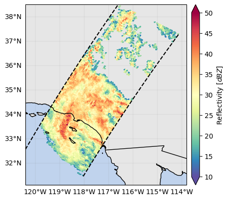
By focusing on a narrow region, it’s possible to better visualize the spatial field:
p = ds[variable].gpm.sel(gpm_id=slice(start_gpm_id, end_gpm_id)).gpm.plot_map()
p.axes.set_title(ds[variable].gpm.title(add_timestep=False))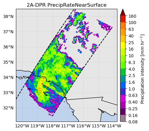
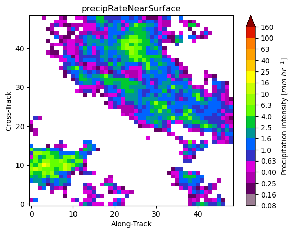
Using the gpm.plot_image method is possible to visualize the data in the so-called “swath scan view”:
ds[variable].gpm.plot_image()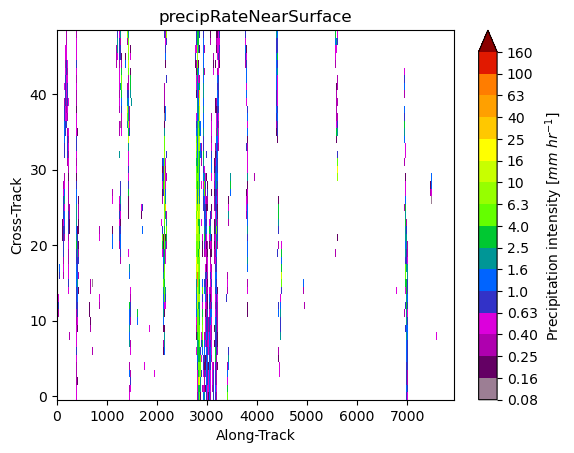
ds[variable].gpm.sel(gpm_id=slice(start_gpm_id, end_gpm_id)).gpm.plot_image()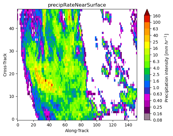
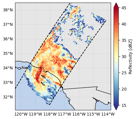
When we visualize different product variables, GPM-API will automatically try to use different appropriate colormaps and colorbars. You can observe this in the following example:
ds_subset = ds.gpm.sel(gpm_id=slice(start_gpm_id, end_gpm_id), radar_frequency="Ku")
p = ds_subset["zFactorFinalNearSurface"].gpm.plot_map()
p = ds_subset["zFactorFinalNearSurface"].gpm.plot_map(
    cmap="RdYlBu_r", vmin=15, vmax=45
)  # ex: enable to modify defaults parameters on the fly
p = ds_subset["flagPrecip"].gpm.plot_map()  # ex: defaults to categorical colorbar
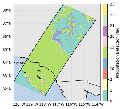
GPM-API provides colormaps and colorbars tailored to GPM product variables with the goal of simplifying the data analysis and make it more reproducible.
The default colormap and colorbar configurations are defined into YAML files into the gpm/etc/colorbars directory of the software.
However, users are free to override, add and/or customize the colorbars configurations using the pycolorbar (https://
The registered colorbar configurations can be displayed using gpm.colorbars.show_colorbars() and the plot_kwargs and cbar_kwargs required to customize the figure can be obtained by calling the gpm.get_plot_kwargs function. Here below we provide an example on how to display DPR precipitation rates estimates using the same colorbar used by NASA to display IMERG liquid precipitation estimates.
plot_kwargs, cbar_kwargs = gpm.get_plot_kwargs("IMERG_Liquid")
ds_subset["precipRateNearSurface"].gpm.plot_map(cbar_kwargs=cbar_kwargs, **plot_kwargs)
<cartopy.mpl.geocollection.GeoQuadMesh at 0x7f66d8c5ce50>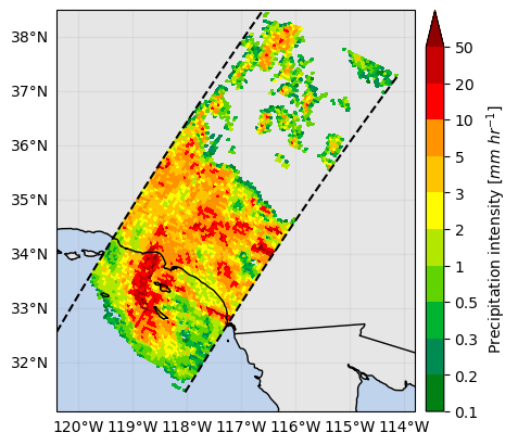
Since GPM Datasets are characterized by multiple dimensions, GPM-API provides the capabilities to generate FacetGrid Cartopy plots following the classical xarray syntax:
ds_subset = ds.gpm.sel(gpm_id=slice(start_gpm_id, end_gpm_id))
# Plot reflectivity at various levels
variable = "zFactorFinal"
da = ds_subset[variable].sel(range=[100, 125, 150, 170])
fc = da.gpm.plot_map(row="radar_frequency", col="range")
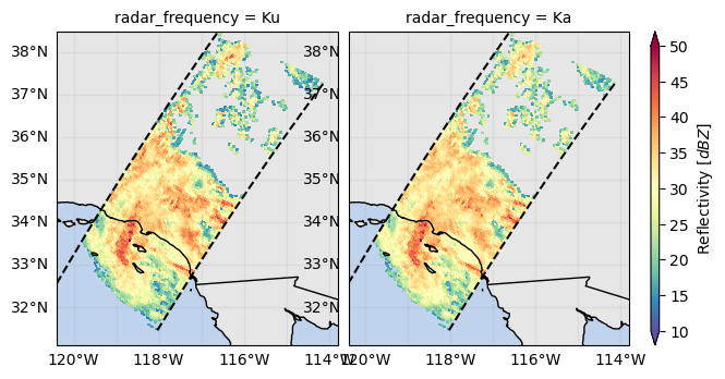
# Surface reflectivity at Ku and Ka band
variable = "zFactorFinalNearSurface"
da = ds_subset[variable]
fc = da.gpm.plot_map(col="radar_frequency", col_wrap=2)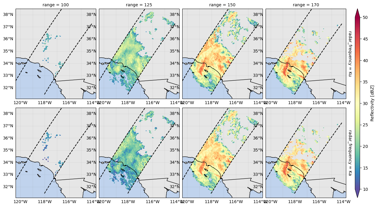
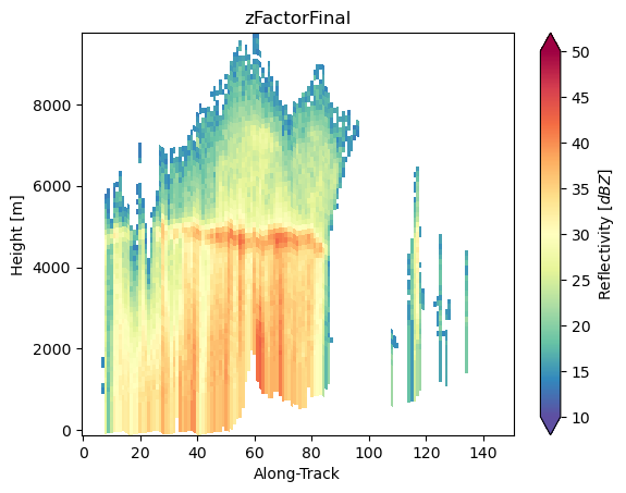
5. Plot Cross-Sections
An easy way to derive a vertical cross-section is to slice the data along the cross-track or along-track dimension.
We can then plot the cross-section calling the gpm.plot_cross_section() method.
ds_subset = ds.gpm.sel(
gpm_id=slice(start_gpm_id, end_gpm_id), radar_frequency="Ku"
).compute()
ds_subset["zFactorFinal"].isel(cross_track=24).gpm.plot_cross_section(zoom=True)
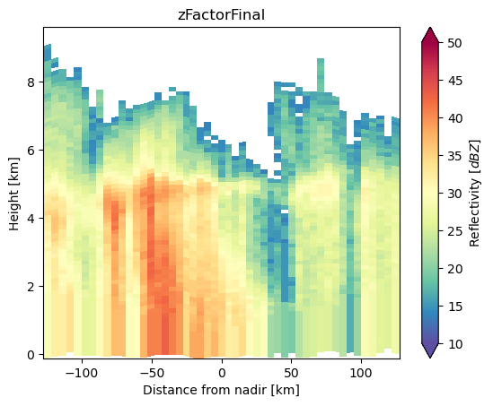
ds_subset["zFactorFinal"].isel(along_track=30).gpm.plot_cross_section(
y="height_km", x="horizontal_distance_km", zoom=True
)
The cross-section transect can be visualized calling the gpm.plot_transect_line method:
ds_transect = ds_subset.isel(cross_track=24)
text_kwargs = {
    "bbox": dict(
        facecolor="white", alpha=0.6, edgecolor="black", boxstyle="round,pad=0.2"
    )
}
p = ds_subset["zFactorFinalNearSurface"].gpm.plot_map()
ds_transect.gpm.plot_transect_line(ax=p.axes, text_kwargs=text_kwargs)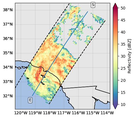
The cross-section variables available in a transect dataset can be listed or selected with gpm.cross_section_variables or gpm.select_cross_section_variables() respectively:
ds_transect = ds_subset.isel(cross_track=24)
print(ds_transect.gpm.cross_section_variables)
ds_transect.gpm.select_cross_section_variables()GPM-API provides accessor methods to facilitate the extraction of cross-section:
- around a point
- between points
- and along a trajectory.
da_cross = ds_subset["zFactorFinal"].gpm.extract_transect_between_points(
    start_point=(-118, 32), end_point=(-118, 36), steps=60
)
da_cross.gpm.plot_cross_section(zoom=True)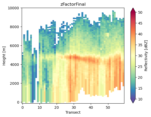
points = np.ones((100, 2))
points[:, 0] = -118
points[:, 1] = np.linspace(32, 36, 100)
da_cross = ds_subset["zFactorFinal"].gpm.extract_transect_at_points(points=points)
da_cross.gpm.plot_cross_section(zoom=True)
da_cross = ds_subset["zFactorFinal"].gpm.extract_transect_around_point(
    point=(-118, 34), azimuth=0, distance=100_000, steps=100
)  # azimuth [0, 360]
da_cross.gpm.plot_cross_section(zoom=True)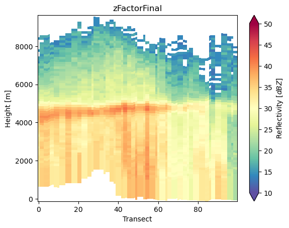
6. Community-based retrievals
GPM-API aims to be a platform where scientist can share their algorithms and retrievals with the community.
Based on the GPM product you are working with, you will have a series of retrievals available to you. For example, GPM-API currently provide the following retrievals for the 2A-DPR product:
ds.gpm.available_retrievals()['EchoDepth',
'EchoTopHeight',
'HailKineticEnergy',
'MESH',
'MESHS',
'POH',
'POSH',
'REFC',
'REFCH',
'SHI',
'VIL',
'VILD',
'bright_band_ratio',
'c_band_tan',
'dfrFinal',
'dfrFinalNearSurface',
'dfrMeasured',
'flagHydroClass',
'flagPrecipitationType',
'gate_resolution',
'gate_volume',
'heightClutterFreeBottom',
'heightRealSurfaceKa',
'heightRealSurfaceKu',
'range_distance_from_ellipsoid',
'range_distance_from_satellite',
'range_resolution',
's_band_cao2013',
'x_band_tan']The gpm.retrieve method enables you to apply specific retrievals to your dataset.
Here below we provide a couple of examples:
ds_subset = ds.gpm.sel(
    gpm_id=slice(start_gpm_id, end_gpm_id), radar_frequency="Ku"
).compute()

ds_subset["EchoTopHeight40dBZ"] = ds_subset.gpm.retrieve("EchoTopHeight", threshold=40)
ds_subset["EchoTopHeight40dBZ"].gpm.plot_map()
<cartopy.mpl.geocollection.GeoQuadMesh at 0x7f66ec31ee50>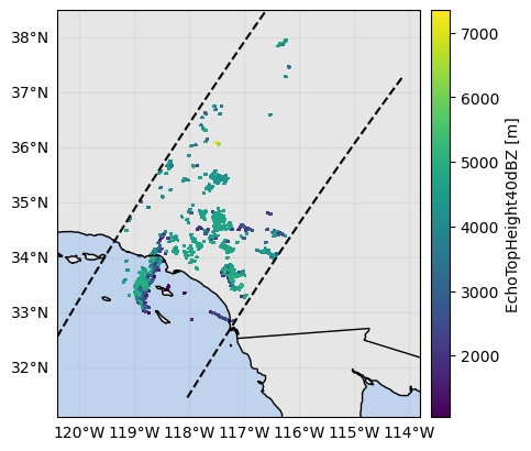
ds_subset["EchoDepthSolid30dBZ"] = ds_subset.gpm.retrieve(
    "EchoDepth", threshold=30, mask_liquid_phase=True
)
ds_subset["EchoDepthSolid30dBZ"].gpm.plot_map()
<cartopy.mpl.geocollection.GeoQuadMesh at 0x7f66ec241910>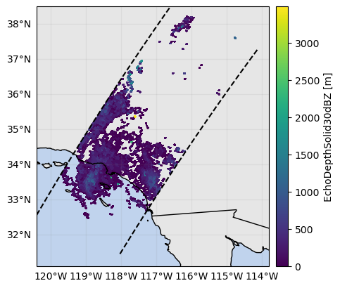
ds_subset["VIL"] = ds_subset.gpm.retrieve("VIL")
ds_subset["VIL"].gpm.plot_map()
<cartopy.mpl.geocollection.GeoQuadMesh at 0x7f66ec24b950>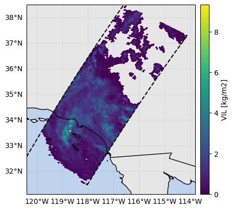
ds_subset["flagPrecipitationType"] = ds_subset.gpm.retrieve(
    "flagPrecipitationType", method="major_rain_type"
)
ds_subset["flagPrecipitationType"].gpm.plot_map()
<cartopy.mpl.geocollection.GeoQuadMesh at 0x7f66daa08590>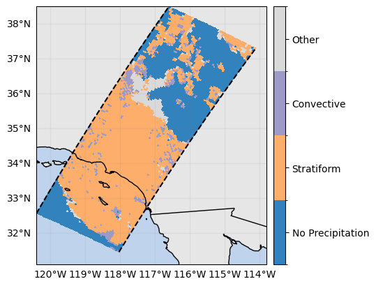
ds_subset["flagHydroClass"] = ds_subset.gpm.retrieve(
    "flagHydroClass"
)  # this return a 3D array !
ds_subset["flagHydroClass"].isel(cross_track=24).gpm.plot_cross_section()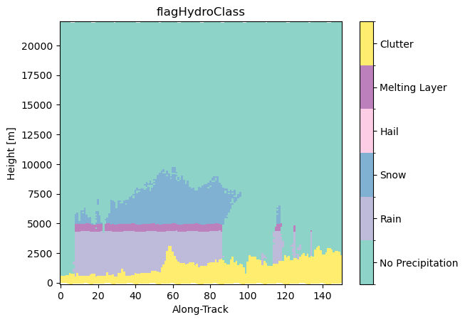
7. Advanced Manipulations
When working with spaceborne radar data, it is often necessary to slice, extract or mask portions of data across the range dimension.
The xarray gpm accessor provides a series of methods to facilitate various tasks.
If you wish to extract the values at specific range gate position varying over each radar beam, you can use the slice_range_at_bin method.
For example, to extract values near the surface where radar gates are not more contaminated by ground clutter, you can use the bin variable "binClutterFreeBottom":
ds_surface = ds_subset.gpm.slice_range_at_bin(
    bins="binClutterFreeBottom"
)  # or ds.gpm.slice_range_at_bin(bins=ds["binClutterFreeBottom"])
ds_surface["precipRate"].gpm.plot_map()  # precipRate is originally a 3D variable !
ds_surface["zFactorFinal"].gpm.plot_map()  # zFactorFinal is originally a 3D variable !
<cartopy.mpl.geocollection.GeoQuadMesh at 0x7f66ec638ed0>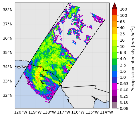
Other slicing methods provide capabilities to retrieve values at a given height, along isothermals, or at the range gates where the minimum, maximum or closest value of a given variable occur:
ds_isothermal = ds_subset.gpm.slice_range_at_temperature(
    273.15
)  # use by default the airTemperature variable
ds_3000 = ds_subset.gpm.slice_range_at_height(3000)
ds_max_z = ds_subset.gpm.slice_range_at_max_value(variable="zFactorFinal")
ds_min_z = ds_subset.gpm.slice_range_at_min_value(variable="zFactorFinal")
ds_at_z_30 = ds_subset.gpm.slice_range_at_value(variable="zFactorFinal", value=30)
If you want to focus your analysis in the portion of radar gates with valid values (e.g., excluding upper atmosphere regions without reflectivities) or values ranging in a specific interval of interest, you can use the subset_range_with_valid_data and subset_range_where_values methods respectively:
ds_valid = ds_subset.gpm.subset_range_with_valid_data(variable="zFactorFinal")
ds_intense = ds_subset.gpm.subset_range_where_values(
    variable="precipRate", vmin=200, vmax=300
)  # mm/hr
print("Range with valid data:", ds_valid["range"].data)
print("Range with intense precipitation:", ds_intense["range"].data)
Range with valid data: [ 93 94 95 96 97 98 99 100 101 102 103 104 105 106 107 108 109 110
111 112 113 114 115 116 117 118 119 120 121 122 123 124 125 126 127 128
129 130 131 132 133 134 135 136 137 138 139 140 141 142 143 144 145 146
147 148 149 150 151 152 153 154 155 156 157 158 159 160 161 162 163 164
165 166 167 168 169 170 171 172 173 174 175 176]
Range with intense precipitation: [166 167 168 169 170 171 172 173 174 175 176]
If you wish to extract radar gates above/below spatially-varying bin position, you can use the extract_dataset_above_bin and extract_dataset_below_bin methods.
Please note that these methods shifts the arrays beam-wise, returning datasets with a new range coordinate and the bin variables updated accordingly.
ds_below_melting_layer = ds_subset.gpm.extract_dataset_below_bin(
    "binBBBottom"
)  # the first new range index corresponds to original binBBBottom
ds_above_melting_layer = ds_subset.gpm.extract_dataset_above_bin(
    "binBBTop"
)  # the last new range index corresponds to original binBBTop
If instead you wish to mask the data above/below or in between radar gates positions, you can use the mask_above_bin, mask_below_bin and mask_between_bins methods:
ds_rain = ds_subset.gpm.mask_above_bin("binZeroDeg")
ds_snow = ds_subset.gpm.mask_below_bin("binZeroDeg")
ds_masked_melting_layer = ds_subset.gpm.mask_between_bins(
    bottom_bins="binBBBottom", top_bins="binBBTop"
)
8. Geospatial Manipulations
GPM-API provides methods to easily spatially subset orbits by extent, country or continent.
Note however, that an area can be crossed by multiple orbits depending on the size of your GPM satellite dataset. In other words, multiple orbit slices in along-track direction can intersect the area of interest.
The method get_crop_slices_by_extent, get_crop_slices_by_country and get_crop_slices_by_continent enable to retrieve the orbit portions intersecting the area of interest.
# Define the variable to display
variable = "precipRateNearSurface"

# Crop by country
list_isel_dict = ds.gpm.get_crop_slices_by_country("United States")
print(list_isel_dict)

# Crop by extent
extent = get_country_extent("United States")
list_isel_dict = ds.gpm.get_crop_slices_by_extent(extent)
print(list_isel_dict)

# Plot the swaths crossing the country
for isel_dict in list_isel_dict:
    da_subset = ds[variable].isel(isel_dict)
    slice_title = da_subset.gpm.title(add_timestep=True)
    p = da_subset.gpm.plot_map()
    p.axes.set_extent(extent)
    p.axes.set_title(label=slice_title)

# Define the variable to display
variable = "precipRateNearSurface"

# Crop around a point (i.e. radar location)
lon = -117.0418
lat = 32.9190
distance = 200_000  # 200 km
list_isel_dict = ds.gpm.get_crop_slices_around_point(
    lon=lon, lat=lat, distance=distance
)
print(list_isel_dict)

extent = get_geographic_extent_around_point(lon=lon, lat=lat, distance=distance)
list_isel_dict = ds.gpm.get_crop_slices_by_extent(extent)
print(list_isel_dict)

# Define ROI coordinates
circle_lons, circle_lats = get_circle_coordinates_around_point(
    lon, lat, radius=distance, num_vertices=360
)

# Plot the swaths crossing the ROI
for isel_dict in list_isel_dict:
    da_subset = ds[variable].isel(isel_dict)
    slice_title = da_subset.gpm.title(add_timestep=True)
    p = da_subset.gpm.plot_map()
    p.axes.plot(circle_lons, circle_lats, "r-", transform=ccrs.Geodetic())
    p.axes.scatter(lon, lat, c="black", marker="X", s=100, transform=ccrs.Geodetic())
    p.axes.set_extent(extent)

# Alternatives if working with a single granule:

# ds_subset = ds.gpm.crop_by_extent(extent)
# ds_subset = ds.gpm.crop_by_country("United States")
[{'along_track': slice(2426, 3805, None)}]
[{'along_track': slice(2426, 3805, None)}]
[{'along_track': slice(2751, 2852, None)}]
[{'along_track': slice(2751, 2852, None)}]
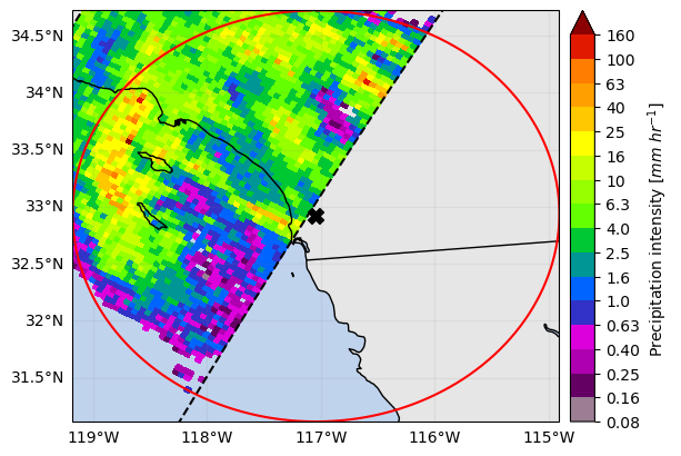
You can also easily obtain the extent around a given point (i.e. ground radar location) using the get_geographic_extent_around_point function and use
the gpm accessor methods get_crop_slices_around_point or crop_around_point to subset your dataset:
# Define the variable to display
variable = "precipRateNearSurface"

# Crop around a point (i.e. radar location)
lon = -117.0418
lat = 32.9190
distance = 200_000  # 200 km
list_isel_dict = ds.gpm.get_crop_slices_around_point(
    lon=lon, lat=lat, distance=distance
)
print(list_isel_dict)

extent = get_geographic_extent_around_point(lon=lon, lat=lat, distance=distance)
list_isel_dict = ds.gpm.get_crop_slices_by_extent(extent)
print(list_isel_dict)

# Define ROI coordinates
circle_lons, circle_lats = get_circle_coordinates_around_point(
    lon, lat, radius=distance, num_vertices=360
)

# Plot the swaths crossing the ROI
for isel_dict in list_isel_dict:
    da_subset = ds[variable].isel(isel_dict)
    slice_title = da_subset.gpm.title(add_timestep=True)
    p = da_subset.gpm.plot_map()
    p.axes.plot(circle_lons, circle_lats, "r-", transform=ccrs.Geodetic())
    p.axes.scatter(lon, lat, c="black", marker="X", s=100, transform=ccrs.Geodetic())
    p.axes.set_extent(extent)

# Alternatives if working with a single granule:

# ds_subset = ds.gpm.crop_around_point(lon=lon, lat=lat, distance=distance)
[{'along_track': slice(2751, 2852, None)}]
[{'along_track': slice(2751, 2852, None)}]
Please keep in mind that you can easily retrieve the extent of a GPM xarray object using the extent method.
The optional argument padding allows to expand/shrink the geographic extent by custom lon/lat degrees, while the size argument allows
to obtain an extent centered on the GPM object with the desired size.
print(da_subset.gpm.extent(padding=0.1))  # expanding
print(da_subset.gpm.extent(padding=-0.1))  # shrinking
print(da_subset.gpm.extent(size=0.5))
print(da_subset.gpm.extent(size=0))  # centroid
Extent(xmin=-120.85270843505859, xmax=-115.86820831298829, ymin=30.720465087890624, ymax=35.94685516357422)
Extent(xmin=-120.6527084350586, xmax=-116.06820831298828, ymin=30.920465087890626, ymax=35.74685516357422)
Extent(xmin=-118.61045837402344, xmax=-118.11045837402344, ymin=33.08366012573242, ymax=33.58366012573242)
Extent(xmin=-118.36045837402344, xmax=-118.36045837402344, ymin=33.33366012573242, ymax=33.33366012573242)
9. Storm Labeling
Using the xarray ximage accessor, it is possible to easily delineate (label) the precipitating areas. The label array is added to the dataset as a new coordinate.
# Retrieve labeled xarray object
label_name = "label"
ds = ds.ximage.label(
    variable="precipRateNearSurface",
    min_value_threshold=1,
    min_area_threshold=5,
    footprint=5,  # assign same label to precipitating areas 5 pixels apart
    sort_by="area",  # "maximum", "minimum", <custom_function>
    sort_decreasing=True,
    label_name=label_name,
)
# Plot full label array
ds[label_name].ximage.plot_labels()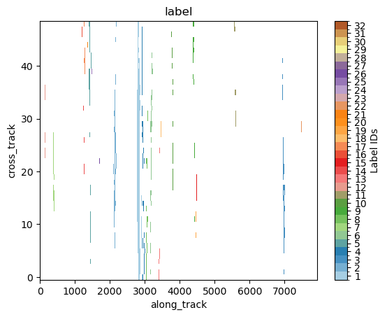
Let’s zoom in a specific region:
gpm.plot_labels(ds[label_name].isel(along_track=slice(2700, 3500)))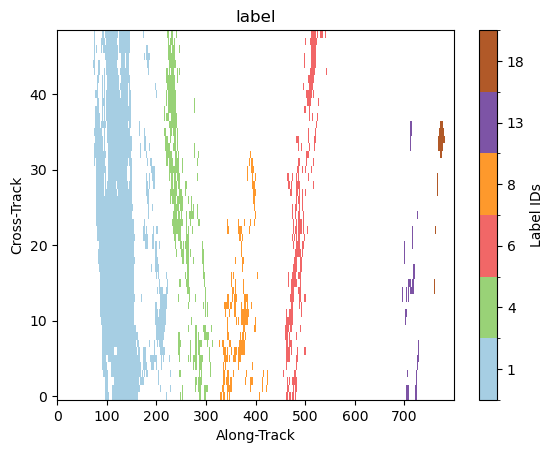
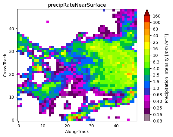
10. Patch Extraction
With the xarray ximage accessor, it is also possible to extract patches around the precipitating areas. Here we provide a minimal example on how to proceed:
# Define the patch generator
da_patch_gen = ds["precipRateNearSurface"].ximage.label_patches(
    label_name=label_name,
    patch_size=(49, 49),
    # Output options
    n_patches=4,
    # Patch extraction Options
    padding=0,
    centered_on="max",
    # Tiling/Sliding Options
    debug=False,
    verbose=False,
)

# # Retrieve list of patches
list_label_patches = list(da_patch_gen)
list_da = [da for label, da in list_label_patches]

# Display patches
gpm.plot_patches(list_label_patches)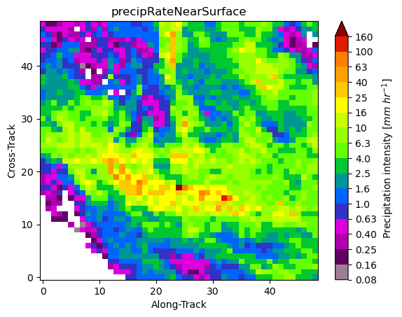
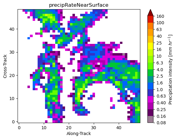
You can exploit the xarray manipulations and FacetGrid capabilities to quickly create the following figure:
list_da_without_coords = [da.drop_vars(["lon", "lat"]) for da in list_da]
da_patch = xr.concat(list_da_without_coords, dim="patch")
da_patch.isel(patch=slice(0, 4)).gpm.plot_image(col="patch", col_wrap=2)
<gpm.visualization.facetgrid.ImageFacetGrid at 0x7f66ec41e450>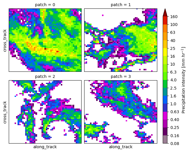
11. Spaceborne/Ground Radar Matching
In this final subsection, we now provide also brief overview on how to match spaceborne (SR) and ground (GR) radar measurements.
A step-by-step guide on the methodology to obtain spatially and temporally coincident radar samples is provided in the Spaceborne-Ground Radar Matching Tutorial, while an applied example is provided in the Spaceborne-Ground Radar Calibration Applied Tutorial.
To start let’s open the NEXRAD ground radar data coincident with the GPM DPR overpass. We have preprocessed the native NEXRAD radar with xradar and uploaded it into Zarr format on the Pythia Cloud Bucket.
bucket_url = "https://js2.jetstream-cloud.org:8001"
fs = fsspec.filesystem("s3", anon=True, client_kwargs=dict(endpoint_url=bucket_url))
file = fs.get_mapper(f"pythia/radar/erad2024/gpm_api/KNKX20230820_221341_V06.zarr")
dt_gr = open_datatree(file, engine="zarr", consolidated=True, chunks={})
display(dt_gr)Now, let’s select the GR sweep to match with GPM DPR.
sweep_idx = 0
sweep_group = f"sweep_{sweep_idx}" # GR sweep (elevation to be used)
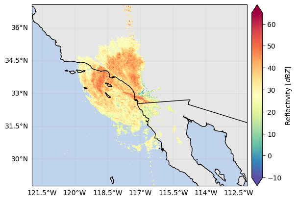
ds_gr = dt_gr[sweep_group].to_dataset().compute()Let’s quickly display the PPI for the horizontally and vertically polarized reflectivity. You will notice that the radar is quite miscalibrated !
ds_gr["DBZH"].where(ds_gr["DBZH"] > -10).xradar_dev.plot_map()
ds_gr["DBZV"] = (ds_gr["DBZH"].gpm.idecibel / ds_gr["ZDR"].gpm.idecibel).gpm.decibel
ds_gr["DBZV"].where(ds_gr["DBZV"] > -10).xradar_dev.plot_map()
# ds_gr["ZDR"].where(ds_gr["DBZV"] > -10).xradar_dev.plot_map()
<cartopy.mpl.geocollection.GeoQuadMesh at 0x7f66da153190>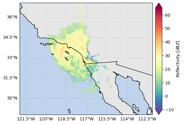
Let’s define some SR/GR volume matching settings ...
radar_band = "S"
beamwidth_gr = 1
z_min_threshold_gr = 0
z_min_threshold_sr = 10
... and then apply the SR/GR volume matching. If the GPM Dataset is not specified, volume_matching automatically download and load the required SR radar data.
gdf_match = volume_matching(
    ds_gr=ds_gr,
    ds_sr=ds,  # optional
    z_variable_gr="DBZH",
    radar_band=radar_band,
    beamwidth_gr=beamwidth_gr,
    z_min_threshold_gr=z_min_threshold_gr,
    z_min_threshold_sr=z_min_threshold_sr,
    min_gr_range=0,
    max_gr_range=150_000,
    # gr_sensitivity_thresholds=None,
    # sr_sensitivity_thresholds=None,
    download_sr=False,  # require NASA accounts and internet connection !
    display_quicklook=True,
)
display(gdf_match)Now let’s display the SR/GR matched/aggregated reflectivities and the preliminary calibration summary:
sr_z_column = f"SR_zFactorFinal_{radar_band}_mean"
gr_z_column = "GR_Z_mean"
# Compare reflectivities
fig = compare_maps(
gdf_match,
sr_column=sr_z_column,
gr_column=gr_z_column,
sr_label="SR Reflectivity (dBz)",
gr_label="GR Reflectivity (dBz)",
cmap="Spectral_r",
unified_color_scale=True,
vmin=15,
# vmax=40
)
fig.tight_layout()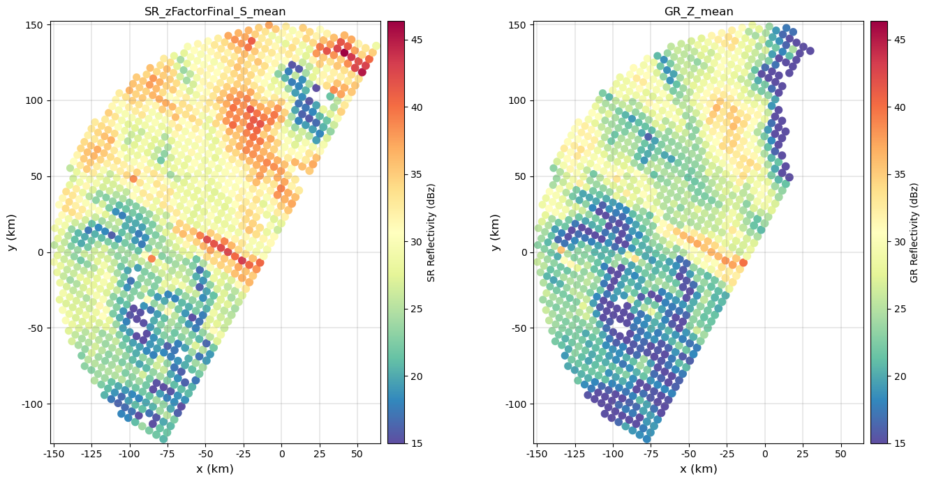
# Display calibration summary
fig = calibration_summary(
    df=gdf_match,
    gr_z_column=gr_z_column,
    sr_z_column=sr_z_column,
    # Histogram options
    bin_width=2,
    # Scatterplot options
    # hue_column="GR_gate_volume_sum",
    hue_column="SR_fraction_clutter",
    # gr_range=[15, 50]
    # sr_range=[15, 50]
    marker="+",
    cmap="Spectral",
)
fig.tight_layout()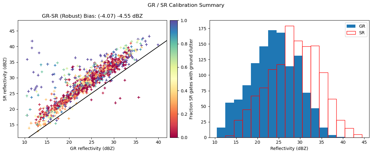
If you are interested in this application, please read the Spaceborne-Ground Radar Calibration Applied Tutorial to investigate and apply filtering criteria to improve the matching process and the calibration of GR data.