wradlib logo png

wradlib - clutter and beamblockage¶

Overview¶

Within this notebook, we will cover:

Reading data using xradar
Clutter detection
Beam Blockage calculation

Prerequisites¶

Concepts	Importance	Notes
Xarray Basics	Helpful	Basic Dataset/DataArray
Matplotlib Basics	Helpful	Basic Plotting
Intro to Cartopy	Helpful	Projections

Time to learn: 10 minutes

Imports¶

import numpy as np
import wradlib as wrl
import matplotlib.pyplot as plt
import xarray as xr
import cartopy
import cartopy.crs as ccrs
import cartopy.feature as cfeature
import xradar as xd
import hvplot
import hvplot.xarray

retrieve data from s3 bucket¶

import os
import urllib.request
from pathlib import Path

# Set the URL for the cloud
URL = "https://js2.jetstream-cloud.org:8001/"
path = "pythia/radar/erad2024"
!mkdir -p data
files = [
    "20240522_MeteoSwiss_ARPA_Lombardia/Data/Xband/DES_VOL_RAW_20240522_1600.nc",
    "wradlib/desio_dem.tif",
]
for file in files:
    file_remote = os.path.join(path, file)
    file_local = os.path.join("data", Path(file).name)
    if not os.path.exists(file_local):
        print(f"downloading, {file_local}")
        urllib.request.urlretrieve(f"{URL}{file_remote}", file_local)

downloading, data/DES_VOL_RAW_20240522_1600.nc

downloading, data/desio_dem.tif

Open CfRadial1 Volume¶

reindex = dict(angle_res=1, direction=1, start_angle=0, stop_angle=360)
dtree = xd.io.open_cfradial1_datatree("data/DES_VOL_RAW_20240522_1600.nc")
display(dtree.load())

Get first sweep¶

swp = (
    dtree["sweep_0"]
    .to_dataset()
    .wrl.georef.georeference(crs=wrl.georef.get_earth_projection())
    .set_coords("sweep_mode")
)
swp.x.attrs = xd.model.get_longitude_attrs()
swp.y.attrs = xd.model.get_latitude_attrs()

display(swp)

Get Digital Elevation Map (DEM)¶

If we have access to the NASA EarthData GESDISC, we can use the BearerToken to retrieve SRTM data corresponding to the actual radar domain. Or we can choose the precompiled GeoTiff.

# extent = [swp.x.min().values, swp.x.max().values, swp.y.min().values, swp.y.max().values]
# import os
# os.environ["WRADLIB_EARTHDATA_BEARER_TOKEN"] = ""
# dem = wrl.io.get_srtm(extent)
# wrl.io.write_raster_dataset("desio_dem.tif", dem)

dem = (
    xr.open_dataset("data/desio_dem.tif", engine="rasterio")
    .isel(band=0)
    .rename(band_data="DEM")
    .reset_coords("band", drop=True)
)
display(dem)

Extract radar parameters¶

radar_parameters = dtree["radar_parameters"]

bw = radar_parameters["radar_beam_width_h"]
bw

Prepare DEM for Polar Processing¶

Here the power of xr.apply_ufunc is shown, a wrapper to xarray-ify numpy functions.

def interpolate_dem(obj, dem, **kwargs):
    dim0 = obj.wrl.util.dim0()

    def wrapper(sx, sy, dx, dy, dem, *args, **kwargs):
        y, x = np.meshgrid(dy, dx)
        rastercoords = np.dstack([x, y])
        polcoords = np.dstack([sx, sy])
        return wrl.ipol.cart_to_irregular_spline(rastercoords, dem, polcoords, **kwargs)

    out = xr.apply_ufunc(
        wrapper,
        obj.x,
        obj.y,
        dem.x,
        dem.y,
        dem,
        input_core_dims=[[dim0, "range"], [dim0, "range"], ["x"], ["y"], ["y", "x"]],
        output_core_dims=[[dim0, "range"]],
        dask="parallelized",
        vectorize=True,
        kwargs=kwargs,
        dask_gufunc_kwargs=dict(allow_rechunk=True),
    )
    out.name = "DEM"
    return obj.assign(DEM=out)

swp = interpolate_dem(swp, dem.DEM, order=3, prefilter=False)

swp.DEM.wrl.vis.plot(cmap="terrain", vmin=0)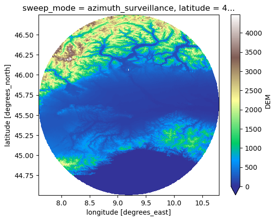

Plot scan strategy¶

nrays = swp.azimuth.size
nbins = swp.range.size
range_res = 300.0
ranges = np.arange(nbins) * range_res
elevs = dtree.root.sweep_fixed_angle.values
sitecoords = (
    dtree.root.longitude.values.item(),
    dtree.root.latitude.values.item(),
    dtree.root.altitude.values.item(),
)

ax = wrl.vis.plot_scan_strategy(
    ranges,
    elevs,
    sitecoords,
    beamwidth=radar_parameters["radar_beam_width_h"].values,
    terrain=None,
)

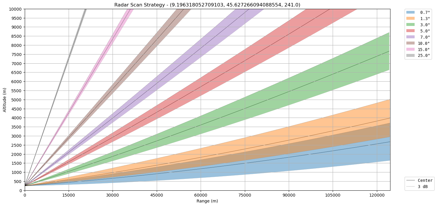
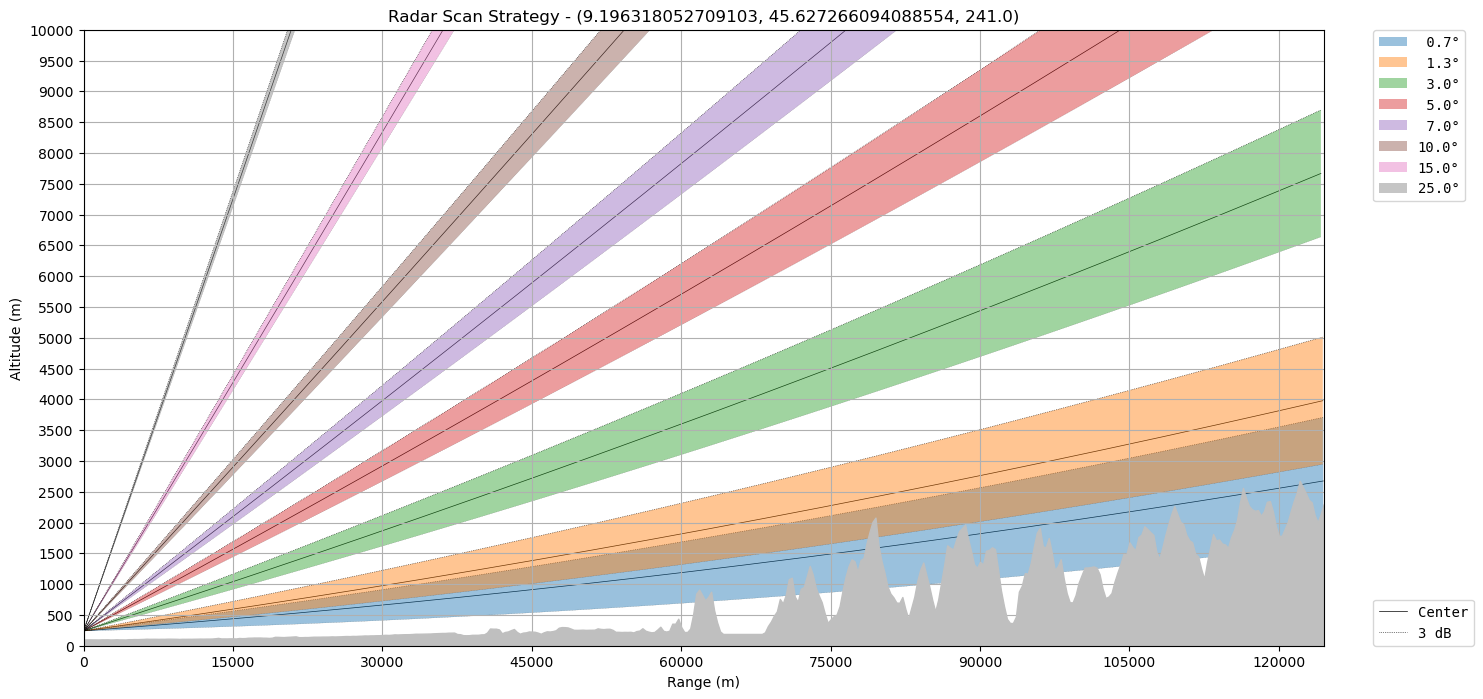
Use terrain=swp.DEM.sel(azimuth=0, method="nearest") to get some arbitrary ray.

ax = wrl.vis.plot_scan_strategy(
    ranges,
    elevs,
    sitecoords,
    beamwidth=radar_parameters["radar_beam_width_h"].values,
    terrain=swp.DEM.sel(azimuth=0, method="nearest"),
)

Calculate clutter map¶

clmap = swp.DBZ_TOT.wrl.classify.filter_gabella(
    wsize=5,
    thrsnorain=0.0,
    tr1=21.0,  # 21.,
    n_p=23.0,  # 23,
    tr2=1.3,
    rm_nans=False,
)
swp = swp.assign({"CMAP": clmap})

Plot Reflectivities, Clutter and Cluttermap¶

fig = plt.figure(figsize=(15, 12))
ax1 = fig.add_subplot(221)
from osgeo import osr

wgs84 = osr.SpatialReference()
wgs84.ImportFromEPSG(4326)
# swp = swp.sel(range=slice(0, 100000)).set_coords("sweep_mode").wrl.georef.georeference(crs=wgs84)
swp.DBZ_TOT.plot(x="x", y="y", ax=ax1, vmin=0, vmax=60)
ax1.set_title("Reflectivity raw")
ax2 = fig.add_subplot(222)
swp.CMAP.plot(x="x", y="y", ax=ax2)
ax2.set_title("Cluttermap")
ax3 = fig.add_subplot(223)
swp.DBZ_TOT.where(swp.CMAP == 1).plot(x="x", y="y", ax=ax3, vmin=0, vmax=60)
ax3.set_title("Clutter")
ax4 = fig.add_subplot(224)
swp.DBZ_TOT.where(swp.CMAP < 1).plot(x="x", y="y", ax=ax4, vmin=0, vmax=60)
ax4.set_title("Reflectivity clutter removed")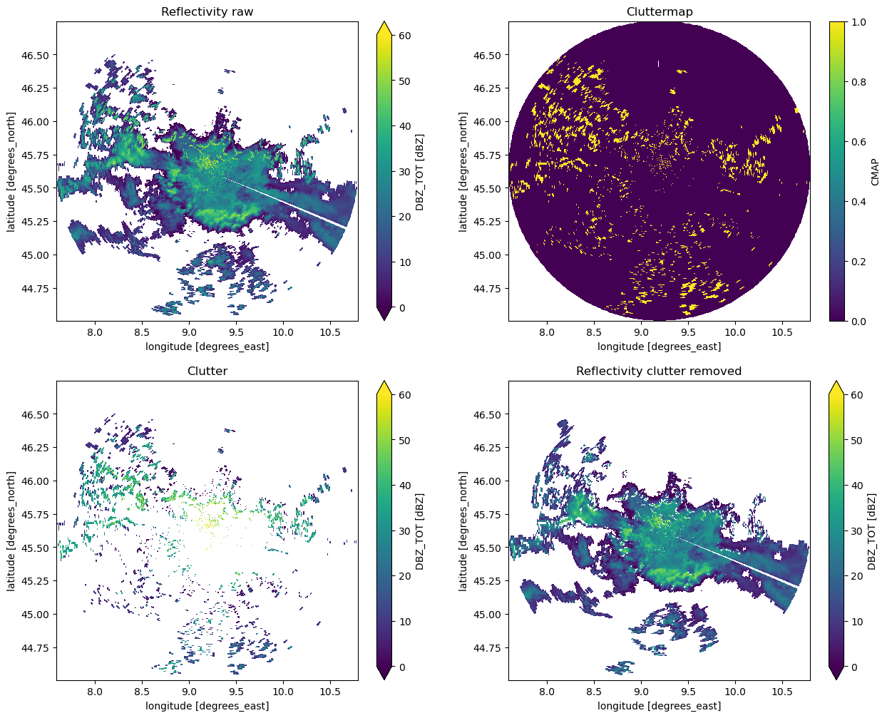

Compare with corrected reflectivity from signal processor¶

plus additional simple RHOHV filter

fig = plt.figure(figsize=(15, 6))
ax1 = fig.add_subplot(121)
swp.DBZ.plot(x="x", y="y", ax=ax1, vmin=0, vmax=60)
ax1.set_title("Reflectivity corr")
ax2 = fig.add_subplot(122)
swp.DBZ_TOT.where((swp.CMAP < 1) & (swp.RHOHV >= 0.8)).plot(
    x="x", y="y", ax=ax2, vmin=0, vmax=60
)
ax2.set_title("Reflectivity clutter removed")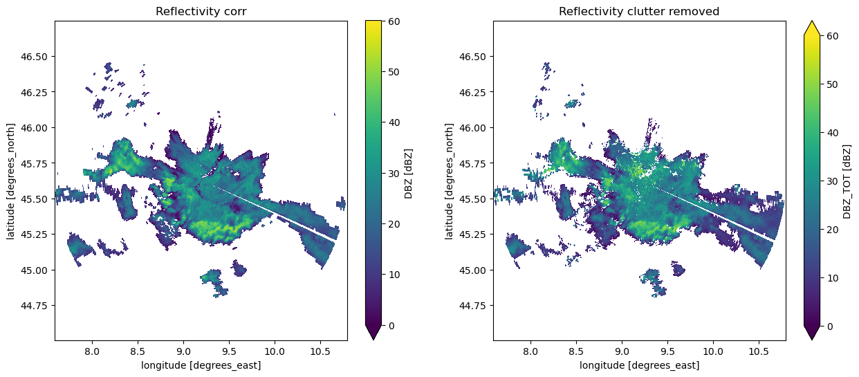

fig = plt.figure(figsize=(8, 5))
ax1 = fig.add_subplot(111)
swp.CMAP.where(swp.CMAP == 1).plot(x="x", y="y", vmin=0, vmax=1, cmap="turbo")
ax1.set_title("Reflectivity corr")
dem.DEM.plot(ax=ax1, zorder=-2, cmap="terrain", vmin=0)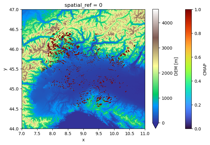

Use hvplot for zooming and panning¶

We need to rechunk the coordinates as hvplot needs chunked variables and coords.

cl = (
    swp.CMAP.where(swp.CMAP == 1)
    .chunk(chunks={})
    .hvplot.quadmesh(
        x="x", y="y", cmap="turbo", width=600, height=500, clim=(0, 1), rasterize=True
    )
)
dm = dem.DEM.chunk(chunks={}).hvplot(
    x="x", y="y", cmap="terrain", width=600, height=500, rasterize=True
)
dm * cl

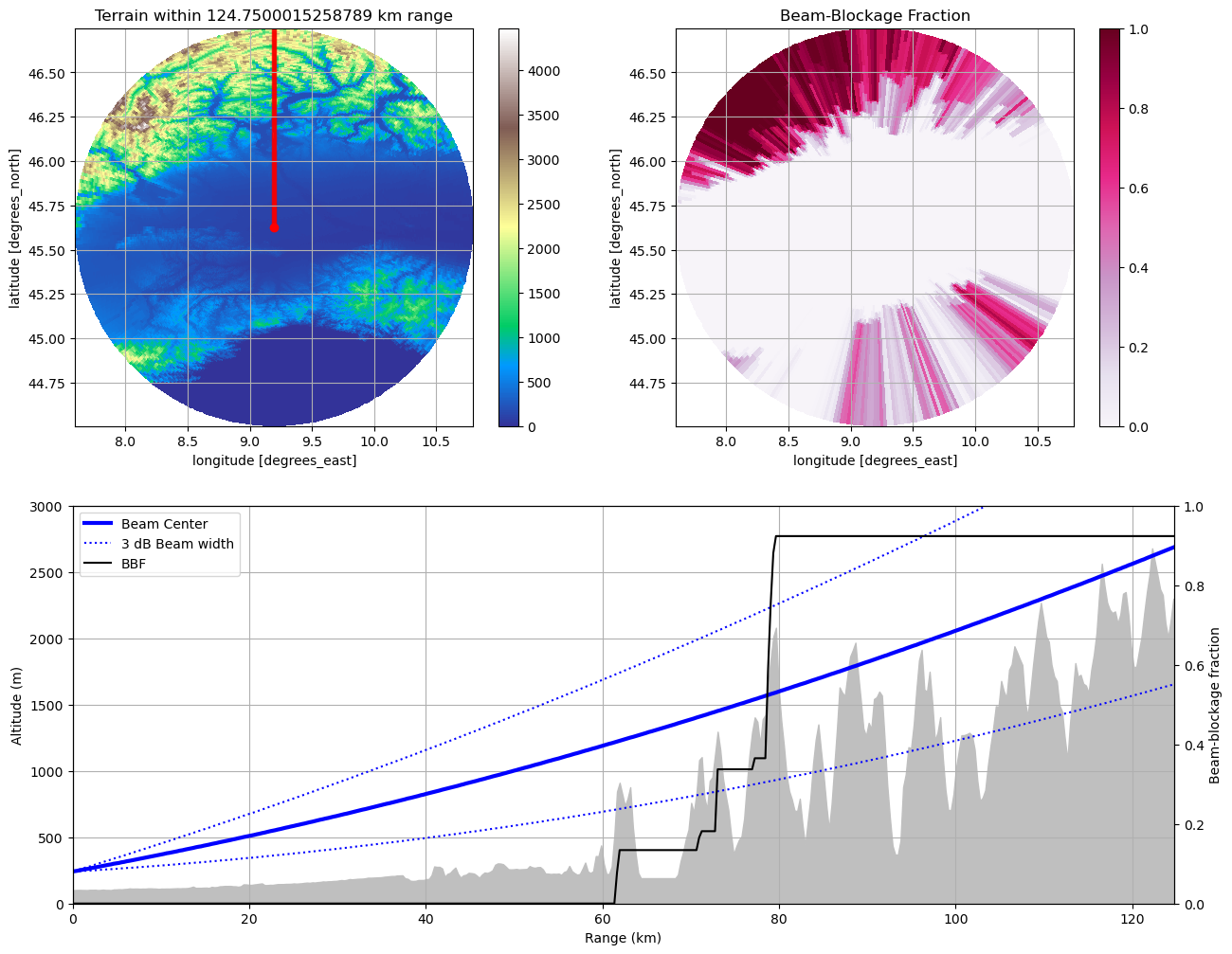
BeamBlockage Calculation¶

Can you xarray-ify the following, too?

beamradius = wrl.util.half_power_radius(swp.range, bw)
PBB = wrl.qual.beam_block_frac(swp.DEM.values, swp.z.values, beamradius)
PBB = np.ma.masked_invalid(PBB)
CBB = wrl.qual.cum_beam_block_frac(PBB)

/srv/conda/envs/notebook/lib/python3.11/site-packages/wradlib/qual.py:184: RuntimeWarning: invalid value encountered in sqrt
  numer = (ya * np.sqrt(a**2 - y**2)) + (a * np.arcsin(ya)) + (np.pi * a / 2.0)
/srv/conda/envs/notebook/lib/python3.11/site-packages/wradlib/qual.py:184: RuntimeWarning: invalid value encountered in arcsin
  numer = (ya * np.sqrt(a**2 - y**2)) + (a * np.arcsin(ya)) + (np.pi * a / 2.0)

swp = swp.assign(
    CBB=(["azimuth", "range"], CBB),
    PBB=(["azimuth", "range"], PBB),
)

# just a little helper function to style x and y axes of our maps
def annotate_map(ax, cm=None, title=""):
    # ticks = (ax.get_xticks() / 1000).astype(int)
    # ax.set_xticklabels(ticks)
    # ticks = (ax.get_yticks() / 1000).astype(int)
    # ax.set_yticklabels(ticks)
    # ax.set_xlabel("Kilometers")
    # ax.set_ylabel("Kilometers")
    if not cm is None:
        plt.colorbar(cm, ax=ax)
    if not title == "":
        ax.set_title(title)
    ax.grid()

import matplotlib as mpl

sitecoords = (swp.longitude.values, swp.latitude.values, swp.altitude.values)
r = swp.range.values
az = swp.azimuth.values

alt = swp.z.values
fig = plt.figure(figsize=(15, 12))

# create subplots
ax1 = plt.subplot2grid((2, 2), (0, 0))
ax2 = plt.subplot2grid((2, 2), (0, 1))
ax3 = plt.subplot2grid((2, 2), (1, 0), colspan=2, rowspan=1)

# azimuth angle
angle = 0

# Plot terrain (on ax1)
dem_pm = swp.DEM.wrl.vis.plot(ax=ax1, cmap=mpl.cm.terrain, vmin=0.0, add_colorbar=False)
swp.sel(azimuth=0, method="nearest").plot.scatter(
    x="x", y="y", marker=".", color="r", alpha=0.2, ax=ax1
)
ax1.plot(swp.longitude.values, swp.latitude.values, "ro")
annotate_map(
    ax1,
    dem_pm,
    "Terrain within {0} km range".format(np.max(swp.range.values / 1000.0) + 0.1),
)

# Plot CBB (on ax2)
cbb = swp.CBB.wrl.vis.plot(ax=ax2, cmap=mpl.cm.PuRd, vmin=0, vmax=1, add_colorbar=False)
annotate_map(ax2, cbb, "Beam-Blockage Fraction")

# Plot single ray terrain profile on ax3
(bc,) = ax3.plot(
    swp.range / 1000.0, swp.z[angle, :], "-b", linewidth=3, label="Beam Center"
)
(b3db,) = ax3.plot(
    swp.range.values / 1000.0,
    (swp.z[angle, :] + beamradius),
    ":b",
    linewidth=1.5,
    label="3 dB Beam width",
)
ax3.plot(swp.range / 1000.0, (swp.z[angle, :] - beamradius), ":b")
ax3.fill_between(swp.range / 1000.0, 0.0, swp.DEM[angle, :], color="0.75")
ax3.set_xlim(0.0, np.max(swp.range / 1000.0) + 0.1)
ax3.set_ylim(0.0, 3000)
ax3.set_xlabel("Range (km)")
ax3.set_ylabel("Altitude (m)")
ax3.grid()

axb = ax3.twinx()
(bbf,) = axb.plot(swp.range / 1000.0, swp.CBB[angle, :], "-k", label="BBF")
axb.set_ylabel("Beam-blockage fraction")
axb.set_ylim(0.0, 1.0)
axb.set_xlim(0.0, np.max(swp.range / 1000.0) + 0.1)


legend = ax3.legend(
    (bc, b3db, bbf),
    ("Beam Center", "3 dB Beam width", "BBF"),
    loc="upper left",
    fontsize=10,
)

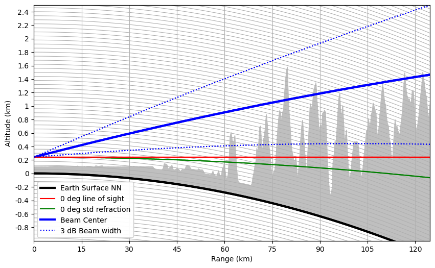
Some EyeCandy¶

def height_formatter(x, pos):
    x = (x - 6370000) / 1000
    fmt_str = "{:g}".format(x)
    return fmt_str


def range_formatter(x, pos):
    x = x / 1000.0
    fmt_str = "{:g}".format(x)
    return fmt_str

fig = plt.figure(figsize=(10, 6))

cgax, caax, paax = wrl.vis.create_cg(fig=fig, rot=0, scale=1)

# azimuth angle
angle = 0

# fix grid_helper
er = 6370000
gh = cgax.get_grid_helper()
gh.grid_finder.grid_locator2._nbins = 80
gh.grid_finder.grid_locator2._steps = [1, 2, 4, 5, 10]

# calculate beam_height and arc_distance for ke=1
# means line of sight
bhe = wrl.georef.bin_altitude(r, 0, sitecoords[2], re=er, ke=1.0)
ade = wrl.georef.bin_distance(r, 0, sitecoords[2], re=er, ke=1.0)
nn0 = np.zeros_like(r)
# for nice plotting we assume earth_radius = 6370000 m
ecp = nn0 + er
# theta (arc_distance sector angle)
thetap = -np.degrees(ade / er) + 90.0

# zero degree elevation with standard refraction
bh0 = wrl.georef.bin_altitude(r, 0, sitecoords[2], re=er)

# plot (ecp is earth surface normal null)
(bes,) = paax.plot(thetap, ecp, "-k", linewidth=3, label="Earth Surface NN")
(bc,) = paax.plot(thetap, ecp + alt[angle, :], "-b", linewidth=3, label="Beam Center")
(bc0r,) = paax.plot(thetap, ecp + bh0, "-g", label="0 deg Refraction")
(bc0n,) = paax.plot(thetap, ecp + bhe, "-r", label="0 deg line of sight")
(b3db,) = paax.plot(
    thetap, ecp + alt[angle, :] + beamradius, ":b", label="+3 dB Beam width"
)
paax.plot(thetap, ecp + alt[angle, :] - beamradius, ":b", label="-3 dB Beam width")

# orography
paax.fill_between(thetap, ecp, ecp + swp.DEM[angle, :], color="0.75")

# shape axes
cgax.set_xlim(0, np.max(ade))
cgax.set_ylim([ecp.min() - 1000, ecp.max() + 2500])
caax.grid(True, axis="x")
cgax.grid(True, axis="y")
cgax.axis["top"].toggle(all=False)
caax.yaxis.set_major_locator(
    mpl.ticker.MaxNLocator(steps=[1, 2, 4, 5, 10], nbins=20, prune="both")
)
caax.xaxis.set_major_locator(mpl.ticker.MaxNLocator())
caax.yaxis.set_major_formatter(mpl.ticker.FuncFormatter(height_formatter))
caax.xaxis.set_major_formatter(mpl.ticker.FuncFormatter(range_formatter))

caax.set_xlabel("Range (km)")
caax.set_ylabel("Altitude (km)")

legend = paax.legend(
    (bes, bc0n, bc0r, bc, b3db),
    (
        "Earth Surface NN",
        "0 deg line of sight",
        "0 deg std refraction",
        "Beam Center",
        "3 dB Beam width",
    ),
    loc="lower left",
    fontsize=10,
)

Summary¶

We’ve just learned how to use $\omega radlib$ ’s Gabella clutter detection for single sweeps. We’ve looked into digital elevation maps and beam blockage calculations.

Resources and references¶

Py-ART and wradlib

Py-ART Basics with Xradar

Py-ART and wradlib

Introduction to GPM-API