This notebook shows how to access hourly rain-gauge precipitation from Serbian surface stations for the same two radar case dates covered in Data Access — Serbian Rainbow Radar (15 May 2014 and 12 August 2017). The data is hosted on the NSF Open Storage Network (OSN) as cloud-optimized Parquet, so every query below is a single pandas call straight against the bucket — no downloads, no credentials, no server.
The layout follows a common open-data pattern used by national hydromet services: a small station catalog plus observations hive-partitioned by station, where the object path itself acts as the index:
s3://nexrad-arco/serbian-stations/
├── stations.parquet                      # station catalog: id, name, lat, lon, altitude
└── precipitation/                        # observations, one partition per station
    ├── station_id=13067/part-0.parquet   # 48 rows: 24 h × 2 event dates
    ├── station_id=13160/part-0.parquet
└── ... # 28 stations total| Access pattern | pandas call | When to use |
|---|---|---|
| One station | read_parquet(".../station_id=13278") | Compare a gauge against the radar gate above it |
| Filtered read | read_parquet(".../precipitation", filters=...) | A few stations / one event, minimal transfer |
| Whole dataset | read_parquet(".../precipitation") | Maps, event totals — it is only ~1,300 rows |
Setup
import fsspec
import matplotlib.pyplot as plt
import pandas as pd

OSN_ENDPOINT = "https://umn1.osn.mghpcc.org"
BUCKET = "nexrad-arco"
PREFIX = "serbian-stations"

STORAGE_OPTIONS = {"anon": True, "client_kwargs": {"endpoint_url": OSN_ENDPOINT}}
Part 1: Browse the bucket
With hive partitioning, the directory tree is the index: each station lives under its own station_id= prefix, so listing the bucket already tells you what can be queried.
fs = fsspec.filesystem(
    "s3", anon=True, client_kwargs={"endpoint_url": OSN_ENDPOINT},
)

for entry in sorted(fs.ls(f"{BUCKET}/{PREFIX}"))[:5]:
    print(entry)
print("...")
partitions = fs.ls(f"{BUCKET}/{PREFIX}/precipitation")
print(f"{len(partitions)} station partitions")
nexrad-arco/serbian-stations/precipitation
nexrad-arco/serbian-stations/stations.parquet
...
28 station partitions
Part 2: Station catalog
The catalog answers “which stations, and where?” — one row per gauge with its WMO-style station_id and coordinates. It is the pivot for everything else: the station_id selects an observation partition, the lat/lon locate the gauge in the radar domain.
stations = pd.read_parquet(
    f"s3://{BUCKET}/{PREFIX}/stations.parquet",
    storage_options=STORAGE_OPTIONS,
)
stations.head()Part 3: Read one station
The most common query — a single gauge’s hourly series, e.g. to compare against the radar gate above it. The station id is the path, so only that partition’s few kilobytes cross the network; the other 27 stations are never touched.
kragujevac = stations.loc[stations["name"] == "Kragujevac"].squeeze()
kragujevac
station_id 13278
name Kragujevac
csv_name Kragujevac
lat 44.027219
lon 20.927769
altitude_m 181.0
Name: 10, dtype: objectobs = pd.read_parquet(
f"s3://{BUCKET}/{PREFIX}/precipitation/station_id={kragujevac.station_id}",
storage_options=STORAGE_OPTIONS,
)
obs.head()Each partition holds both event dates (24 hourly rows each), distinguished by the date column:
obs.groupby("date")["precip_mm"].agg(["count", "sum", "max"])Part 4: Filtered reads with partition pruning
Reading the dataset root with filters= lets pandas/pyarrow prune partitions before any data is fetched: only the directories matching station_id are downloaded, and the date filter is applied from parquet statistics inside them. The same code works unchanged on archives a million times this size — this is how national hydromet services publish decades of station records as queryable open data.
subset = pd.read_parquet(
    f"s3://{BUCKET}/{PREFIX}/precipitation",
    filters=[
        ("station_id", "in", [13278, 13388]),  # Kragujevac, Niš
        ("date", "==", "2017-08-12"),
    ],
    storage_options=STORAGE_OPTIONS,
)
subset.groupby(["station_id", "station_name"], observed=True)["precip_mm"].sum()
station_id station_name
13278 Kragujevac 27.6
13388 Niš 2.8
Name: precip_mm, dtype: float64Note the hive key comes back as a categorical column — pandas materializes station_id from the directory names rather than reading it from the files.
Part 5: Join observations with the catalog
Merging on station_id tags every observation with its coordinates — the entry point for gauge-to-radar comparison: pick a gauge, use its lat/lon to select the radar gate above it, then compare the two time series.
precip = pd.read_parquet(
    f"s3://{BUCKET}/{PREFIX}/precipitation",
    storage_options=STORAGE_OPTIONS,
)

totals = (
    precip.groupby(["station_id", "date"], observed=True)["precip_mm"]
    .sum()
    .reset_index()
    .merge(stations[["station_id", "name", "lat", "lon"]], on="station_id")
)
totals.sort_values("precip_mm", ascending=False).head()Part 6: Map the event totals
24-hour accumulated precipitation at every gauge for each case date — the surface-station view of the storms seen by the FGora and Jastrebac radars.
fig, axs = plt.subplots(1, 2, figsize=(12, 5), sharex=True, sharey=True)

for ax, (date, day) in zip(axs, totals.groupby("date")):
    sc = ax.scatter(
        day["lon"], day["lat"], c=day["precip_mm"],
        cmap="Blues", edgecolor="k", s=80, vmin=0,
    )
    ax.set_title(f"{date} — 24 h accumulation")
    ax.set_xlabel("Longitude [°E]")
    fig.colorbar(sc, ax=ax, label="precip [mm]")

axs[0].set_ylabel("Latitude [°N]")
fig.tight_layout()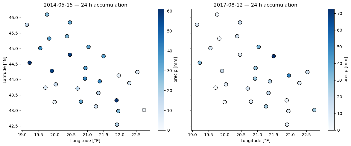
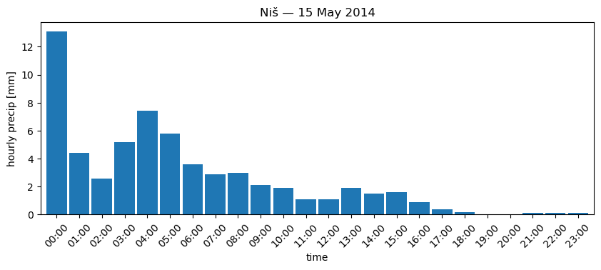
And the hourly evolution at the wettest gauge of the 2014 event:
wettest = totals[totals["date"] == "2014-05-15"].nlargest(1, "precip_mm").squeeze()

series = pd.read_parquet(
    f"s3://{BUCKET}/{PREFIX}/precipitation/station_id={wettest.station_id}",
    storage_options=STORAGE_OPTIONS,
)
series = series[series["date"] == "2014-05-15"].set_index("time")

hourly = series["precip_mm"]
hourly.index = hourly.index.strftime("%H:%M")
hourly.plot(
    kind="bar", figsize=(10, 3.5), width=0.9, rot=45,
    ylabel="hourly precip [mm]",
    title=f"{wettest['name']} — 15 May 2014",
);
Summary
| Raw CSV / Excel | Cloud-optimized Parquet | |
|---|---|---|
| Location | scattered files, per-event layout | s3://nexrad-arco/serbian-stations/ |
| Format | wide tables, mixed encodings, ambiguous dates | tidy long, typed schema, UTC timestamps |
| Access | download + clean every time | one pd.read_parquet("s3://...") call |
| Station lookup | column-header string matching | station_id partition path or filter |
| Coordinates | separate spreadsheet, mismatched names | catalog joined on station_id |
| Coverage | — | 28 stations × 2 events × 24 h (1,344 obs) |
References
NSF Open Storage Network — the bucket host
Apache Parquet — columnar storage format
pandas
read_parquet— includingfiltersandstorage_optionsHive partitioning — directory-based dataset layout in Apache Arrow
RHMSS — Republic Hydrometeorological Service of Serbia, data provider