Py-ART Gridding¶

Overview¶

Within this notebook, we will cover:

What is gridding and why is it important?
An overview of gridding with Py-ART
Test out a different gridding routine
Apply Gridding to a Selection of Files

Prerequisites¶

Concepts	Importance	Notes
Py-ART Basics	Helpful	Basic features
Intro to Cartopy	Helpful	Basic features
Matplotlib Basics	Helpful	Basic plotting
NumPy Basics	Helpful	Basic arrays

Time to learn: 15 minutes

Imports¶

import os
from pathlib import Path
import glob
import warnings

import cartopy.crs as ccrs
import matplotlib.pyplot as plt
import fsspec
import re
import pyart
from pyart.testing import get_test_data
from datetime import datetime
import xarray as xr

OSN_ENDPOINT = "https://umn1.osn.mghpcc.org"
BUCKET = "nexrad-arco"
warnings.filterwarnings('ignore')


## You are using the Python ARM Radar Toolkit (Py-ART), an open source
## library for working with weather radar data. Py-ART is partly supported
## by the U.S. Department of Energy Office of Science as part of
## the Atmospheric Radiation Measurement (ARM) User Facility.
##
## If you use this software to prepare a publication, please cite:
##
##     JJ Helmus and SM Collis, JORS 2016, doi: 10.5334/jors.119

What is gridding and why is it important?¶

Antenna vs. Cartesian Coordinates¶

Radar data, by default, is stored in a polar (or antenna) coordinate system, with the data coordinates stored as an angle (ranging from 0 to 360 degrees with 0 == North), and a radius from the radar, and an elevation which is the angle between the ground and the ground.

This format can be challenging to plot, since it is scan/radar specific. Also, it can make comparing with model data, which is on a lat/lon grid, challenging since one would need to transform the model daa cartesian coordinates to polar/antenna coordiantes.

Fortunately, PyART has a variety of gridding routines, which can be used to grid your data to a Cartesian grid. Once it is in this new grid, one can easily slice/dice the dataset, and compare to other data sources.

Why is Gridding Important?¶

Gridding is essential to combining multiple data sources (ex. multiple radars), and comparing to other data sources (ex. model data). There are also decisions that are made during the gridding process that have a large impact on the regridded data - for example:

What resolution should my grid be?
Which interpolation routine should I use?
How smooth should my interpolated data be?

While there is not always a right or wrong answer, it is important to understand the options available, and document which routine you used with your data! Also - experiment with different options and choose the best for your use case!

An overview of gridding with Py-ART¶

Let’s dig into the regridding process with PyART!

Read in the Data and Plot the Data¶

Read in a sample file from the Fruska Gora (FGora) radar¶

Our data is formatted as a Rainbow file used by Leonardo radars. We will download the data locally so that Py-ART’s Rainbow reader can read the files.

from pathlib import Path
fs = fsspec.filesystem(
    "s3", anon=True, client_kwargs={"endpoint_url": OSN_ENDPOINT},
)
fgora_raw = sorted(fs.glob(f"{BUCKET}/fgora_vol/**/*.vol"))
download_dir = Path("data/fgora_sample")
download_dir.mkdir(parents=True, exist_ok=True)

sample_ts = "2014051500012000"
for remote in [f for f in fgora_raw if sample_ts in f]:
    local = download_dir / Path(remote).name
    if not local.exists():
        fs.get(remote, str(local))
    print(f"  {local.name}")

  2014051500012000V.vol
  2014051500012000W.vol
  2014051500012000dBZ.vol

  2014051500012000dBuZ.vol

radar = pyart.aux_io.read_rainbow_wrl('data/fgora_sample/2014051500012000dBZ.vol')

Let’s plot up quick look of reflectivity, at the lowest elevation scan (closest to the ground)

fig = plt.figure(figsize=[6, 6])
display = pyart.graph.RadarDisplay(radar)
display.plot_ppi('reflectivity', 
                 cmap='HomeyerRainbow')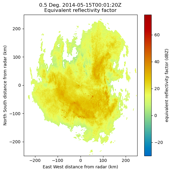

As mentioned before, the dataset is currently in the antenna coordinate system measured as distance from the radar

Setup our Gridding Routine with `pyart.map.grid_from_radars()`¶

Py-ART has the Grid object which has characteristics similar to that of the Radar object, except that the data are stored in Cartesian coordinates instead of the radar’s antenna coordinates.

pyart.core.Grid?

We can transform our data into this grid object, from the radars, using pyart.map.grid_from_radars().

Beforing gridding our data, we need to make a decision about the desired grid resolution and extent. For example, one might imagine a grid configuration of:

Grid extent/limits
- 20 km in the x-direction (north/south)
- 20 km in the y-direction (west/east)
- 15 km in the z-direction (vertical)
500 m spatial resolution

The pyart.map.grid_from_radars() function takes the grid shape and grid limits as input, with the order (z, y, x).

Let’s setup our configuration, setting our grid extent first, with the distance measured in meters

z_grid_limits = (0.,15_000.)
y_grid_limits = (-150_000.,150_000.)
x_grid_limits = (-150_000.,150_000.)

Now that we have our grid limits, we can set our desired resolution (again, in meters)

grid_resolution = 500

Let’s compute our grid shape - using the extent and resolution to compute the number of grid points in each direction.

def compute_number_of_points(extent, resolution):
    return int((extent[1] - extent[0])/resolution)

Now that we have a helper function to compute this, let’s apply it to our vertical dimension

z_grid_points = compute_number_of_points(z_grid_limits, grid_resolution)
z_grid_points

30

We can apply this to the horizontal (x, y) dimensions as well.

x_grid_points = compute_number_of_points(x_grid_limits, grid_resolution)
y_grid_points = compute_number_of_points(y_grid_limits, grid_resolution)

print(z_grid_points,
      y_grid_points,
      x_grid_points)

30 600 600

Use our configuration to grid the data!¶

Now that we have the grid shape and grid limits, let’s grid up our radar!

grid = pyart.map.grid_from_radars(radar,
                                  grid_shape=(z_grid_points,
                                              y_grid_points,
                                              x_grid_points),
                                  grid_limits=(z_grid_limits,
                                               y_grid_limits,
                                               x_grid_limits),
                                  fields=['reflectivity'],
                                  min_radius=500.
                                 )
grid

<pyart.core.grid.Grid at 0x7f9001bb5be0>

We now have a pyart.core.Grid object!

Plot up the Grid Object¶

Plot a horizontal view of the data¶

We can use the GridMapDisplay from pyart.graph to visualize our regridded data, starting with a horizontal view (slice along a single vertical level)

display = pyart.graph.GridMapDisplay(grid)
display.plot_grid('reflectivity',
                  level=3,
                  vmin=-20,
                  vmax=60,
                  cmap='HomeyerRainbow')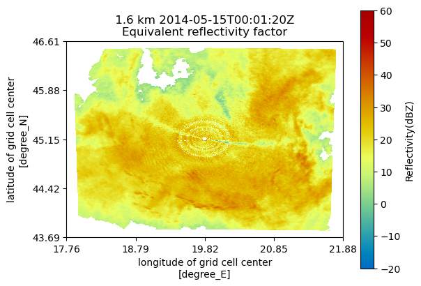

Plot a Latitudinal Slice¶

We can also slice through a single latitude or longitude!

display.plot_latitude_slice('reflectivity',
                            lat=45.15,
                            vmin=-20,
                            vmax=60,
                            cmap='HomeyerRainbow')
plt.xlim([-20, 20]);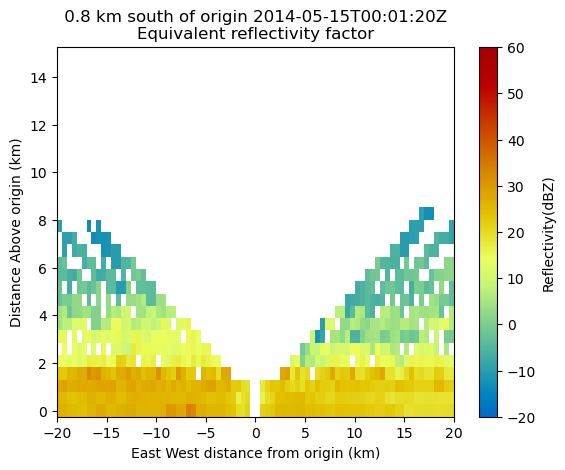

Plot with Xarray¶

Another neat feature of the Grid object is that we can transform it to an xarray.Dataset!

ds = grid.to_xarray()
ds

Now, our plotting routine is a one-liner, starting with the horizontal slice:

ds.isel(z=2).reflectivity.plot(cmap='HomeyerRainbow',
                               vmin=-20,
                               vmax=60);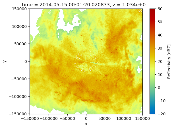

And a vertical slice at a given y dimension (latitude)

ds.sel(y=-3000,
       method='nearest').reflectivity.plot(cmap='HomeyerRainbow',
                                           vmin=-20,
                                           vmax=60);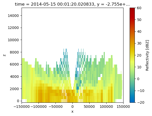

Try a Different Gridding Technique¶

In the previous section, we used the Barnes interpolation technique for interpolating the radar data to Cartesian coordinates. Such an interpolation, while producing smoother grids, can blur out mesoscale phenomena that occur on the scale of the grid resolution such as gust fronts and hail cores. Therefore, to capture these more extreme events, a nearest neighbor interpolation is desired to capture these events at the expense of a noisier grid.

nearest_grid = pyart.map.grid_from_radars(radar,
                                  grid_shape=(z_grid_points,
                                              y_grid_points,
                                              x_grid_points),
                                  grid_limits=(z_grid_limits,
                                               y_grid_limits,
                                               x_grid_limits),
                                  fields=['reflectivity'],
                                  weighting_function='Nearest',
                                  min_radius=500.
                                 )

display.plot_latitude_slice('reflectivity',
                            lat=45.1,
                            vmin=-20,
                            vmax=60,
                            cmap='HomeyerRainbow')
plt.xlim([-20, 20]);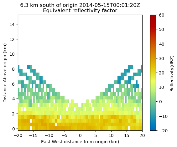

Apply Gridding to a Selection of Files¶

We would like to apply our gridding transformation to an entire list of files, that will enable tracking in future notebooks (ex. tobac). We need to:

Setup a function to grid our data (including saving it to disk)
Provide a list of files to grid

def grid_radar_data(infile, outdir, grid_resolution=500):
    """
    Parameters
    ==========
    infile: string, path to file to be gridded
    outdir: string, path to directory to save to
    grid_resolution: int, desired resolution of field in meters
    
    Returns
    =======
    print statement with saved file
    """

    # Read the data
    radar = pyart.aux_io.read_rainbow_wrl(infile)
    
    # Configure the bounds + compute points
    z_grid_limits = (0.,15_000.)
    y_grid_limits = (-150_000.,150_000.)
    x_grid_limits = (-150_000.,150_000.)
    x_grid_points = compute_number_of_points(x_grid_limits, grid_resolution)
    y_grid_points = compute_number_of_points(y_grid_limits, grid_resolution)
    z_grid_points = compute_number_of_points(z_grid_limits, grid_resolution)
    
    
    # Grid the radar data
    grid = pyart.map.grid_from_radars(radar,
                                  grid_shape=(z_grid_points,
                                              y_grid_points,
                                              x_grid_points),
                                  grid_limits=(z_grid_limits,
                                               y_grid_limits,
                                               x_grid_limits),
                                  fields=['reflectivity'],
                                  weighting_function='Nearest',
                                  min_radius=grid_resolution
                                 )
    
    infile_path = Path(infile)
    os.makedirs(outdir, exist_ok=True)
    outfile = f"{outdir}/{infile_path.stem}.nc"
    
    # Save to disk
    grid.to_xarray().to_netcdf(outfile, mode='w')
    print(f"Done gridding + saving {outfile}")
    return outfile

fs = fsspec.filesystem(
    "s3", anon=True, client_kwargs={"endpoint_url": OSN_ENDPOINT},
)

# Can replace this prefix to jastrebac_vol get the Jastrebac radar
prefix = "fgora_vol"
files = sorted(fs.glob(f"{BUCKET}/{prefix}/**/*.vol"))
pat = re.compile(r'/(\d{14})\d{2}[A-Za-z]+\.vol$')
times = sorted({m.group(1) for f in files if (m := pat.search(f))})
dBz_files = [x for x in files if "dBZ" in x]

def download_file(remote, download_dir=Path("data/fgora_sample")):
    local = download_dir / Path(remote).name
    if not local.exists():
        fs.get(remote, str(local))
    return str(local)

downloaded_files = [download_file(file) for file in dBz_files]
# Let's just target a single date. We have 2014-05-15, 2017-08-12, and 2026-05-12
data_date = "20140515"
downloaded_files = [x for x in downloaded_files if data_date in x]

gridded_data = [grid_radar_data(file,
                                "../../data/fgora/gridded_dBZ/") for file in downloaded_files]

Done gridding + saving ../../data/fgora/gridded_dBZ//2014051500012000dBZ.nc

Done gridding + saving ../../data/fgora/gridded_dBZ//2014051500062000dBZ.nc

Done gridding + saving ../../data/fgora/gridded_dBZ//2014051500112000dBZ.nc

Done gridding + saving ../../data/fgora/gridded_dBZ//2014051500162000dBZ.nc

Done gridding + saving ../../data/fgora/gridded_dBZ//2014051500212000dBZ.nc

Done gridding + saving ../../data/fgora/gridded_dBZ//2014051500262000dBZ.nc

Done gridding + saving ../../data/fgora/gridded_dBZ//2014051500312000dBZ.nc

Done gridding + saving ../../data/fgora/gridded_dBZ//2014051500362000dBZ.nc

Done gridding + saving ../../data/fgora/gridded_dBZ//2014051500412000dBZ.nc

Done gridding + saving ../../data/fgora/gridded_dBZ//2014051500462000dBZ.nc

Done gridding + saving ../../data/fgora/gridded_dBZ//2014051500512000dBZ.nc

Done gridding + saving ../../data/fgora/gridded_dBZ//2014051500562000dBZ.nc

Done gridding + saving ../../data/fgora/gridded_dBZ//2014051501012000dBZ.nc

Done gridding + saving ../../data/fgora/gridded_dBZ//2014051501062000dBZ.nc

Done gridding + saving ../../data/fgora/gridded_dBZ//2014051501112000dBZ.nc

Done gridding + saving ../../data/fgora/gridded_dBZ//2014051501161900dBZ.nc

Done gridding + saving ../../data/fgora/gridded_dBZ//2014051501212000dBZ.nc

Done gridding + saving ../../data/fgora/gridded_dBZ//2014051501262000dBZ.nc

Done gridding + saving ../../data/fgora/gridded_dBZ//2014051501311900dBZ.nc

Done gridding + saving ../../data/fgora/gridded_dBZ//2014051501362000dBZ.nc

Done gridding + saving ../../data/fgora/gridded_dBZ//2014051501412000dBZ.nc

Done gridding + saving ../../data/fgora/gridded_dBZ//2014051501462000dBZ.nc

Done gridding + saving ../../data/fgora/gridded_dBZ//2014051501512000dBZ.nc

Done gridding + saving ../../data/fgora/gridded_dBZ//2014051501562000dBZ.nc

Done gridding + saving ../../data/fgora/gridded_dBZ//2014051502012000dBZ.nc

Read in the Gridded Data and Plot It¶

Now that we have our output, we can read all of it into the same xarray.Dataset, and visualize our data!

ds = xr.open_mfdataset(gridded_data).squeeze()

ds.reflectivity.isel(z=2).plot(x='x',
                               y='y',
                               col='time',
                               vmin=-20,
                               vmax=70,
                               cmap='ChaseSpectral',
                               col_wrap=5);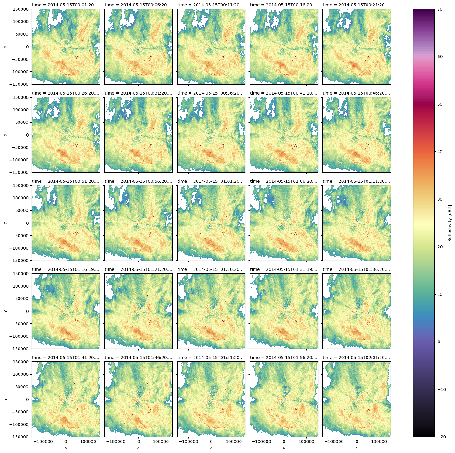

Summary¶

Within this notebook, we covered the basics of gridding radar data using pyart, including:

What we mean by gridding and why is it matters
Configuring your gridding routine
Visualize gridded radar data

What’s Next¶

In the next few notebooks, we walk through applying data cleaning methods, and advanced visualization methods!

Resources and References¶

Py-ART essentials links:

Py-ART Gridding