Calculating ZDR offsets with xradar and Py-ART¶

Overview¶

Differential reflectivity ( $Z_{DR}$ ) is the ratio, in decibels, of the reflectivity at horizontal polarization to that at vertical polarization. It is one of the most powerful dual-polarization variables — but it is also one of the most sensitive to calibration. A system $Z_{DR}$ bias of a few tenths of a dB propagates directly into rainfall estimates, hydrometeor classification, and attenuation correction, so before $Z_{DR}$ can be used quantitatively the system offset must be found and removed.

This notebook demonstrates the classic light-rain / “spherical-drop” method for estimating the $Z_{DR}$ offset. In light stratiform rain the drops are small and nearly spherical, so their intrinsic $Z_{DR}$ is close to 0 dB. If we isolate those gates and the observed $Z_{DR}$ there sits at some non-zero value, that value is the system offset.

Within this notebook, we will cover:

Reading ARCO (icechunk/Zarr) dual-pol data into xarray and bridging it into Py-ART
Using cross-correlation ratio ( $\rho_{HV}$ ) and reflectivity ( $Z_H$ ) to find areas of small, spherical droplets
The statistical calculation of the $Z_{DR}$ offset
Adding the new offset-corrected $Z_{DR}$ field back to the radar object

Prerequisites¶

Concepts	Importance	Notes
Data Access — Serbian Rainbow Radar	Required	How the ARCO store is opened
Py-ART Basics	Helpful	Basic features
Matplotlib Basics	Helpful	Basic plotting
NumPy Basics	Helpful	Basic arrays

Time to learn: 45 minutes

Imports¶

import warnings

import matplotlib.pyplot as plt
import numpy as np
import pandas as pd

import cmweather  # registers HomeyerRainbow, plasmidis, ChaseSpectral colormaps
import icechunk
import xarray as xr
import pyart
from pyart.xradar import Xradar

OSN_ENDPOINT = "https://umn1.osn.mghpcc.org"
BUCKET = "nexrad-arco"

warnings.filterwarnings("ignore")


## You are using the Python ARM Radar Toolkit (Py-ART), an open source
## library for working with weather radar data. Py-ART is partly supported
## by the U.S. Department of Energy Office of Science as part of
## the Atmospheric Radiation Measurement (ARM) User Facility.
##
## If you use this software to prepare a publication, please cite:
##
##     JJ Helmus and SM Collis, JORS 2016, doi: 10.5334/jors.119

Claim Data¶

We use the ARCO data provided in Data Access — Serbian Rainbow Radar. Please refer to this notebook for the details of access. We work with the Jastrebac dual-pol radar, whose 2017 and 2026 volumes live in the jastrebac_500m store (500 m gates, 12 sweeps, 360 azimuths).

# prefix = "jastrebac_250m"  # dual-pol, 12 × 360 × 1000, 2014 only
prefix = "jastrebac_500m"  # dual-pol, 12 × 360 × 500,  2017 + 2026

storage = icechunk.s3_storage(
    bucket=BUCKET,
    prefix=prefix,
    endpoint_url=OSN_ENDPOINT,
    region="us-east-1",
    anonymous=True,
    force_path_style=True,
)
repo = icechunk.Repository.open(storage)

The volumes are indexed along a vcp_time dimension whose CF units string ("nanoseconds since 1950-01-01") is not one xarray decodes automatically, so we open with decode_times=False and convert the time axis by hand.

dtree = xr.open_datatree(
    repo.readonly_session("main").store,
    engine="zarr",
    consolidated=False,
    chunks={},
    decode_times=False,
)
root = next(iter(dtree.keys())).split("/")[0]

# Decode "nanoseconds since 1950-01-01" -> datetime64[ns]
vcp_time = (
    np.datetime64("1950-01-01")
    + np.asarray(dtree[root]["vcp_time"].values).astype("int64").astype("timedelta64[ns]")
)
print(f"Task     : /{root}")
print(f"Volumes  : {vcp_time.size}  ({pd.Timestamp(vcp_time.min())} → {pd.Timestamp(vcp_time.max())})")
print(f"Sweeps   : {len(list(dtree[root].children))}")
dtree

Task     : /JSTB_250_Dp_leto
Volumes  : 71  (2017-08-12 15:05:06 → 2026-05-12 09:55:07)
Sweeps   : 12

Pick a volume with widespread light rain¶

The spherical-drop method needs a scan with plenty of stratiform echo. We score every volume by the fraction of low-level gates exceeding 10 dBZ and take the best one.

dbzh0 = dtree[f"{root}/sweep_0"].to_dataset()["DBZH"]  # (vcp_time, azimuth, range)
coverage = (dbzh0 > 10).mean(dim=["azimuth", "range"]).values
k = int(np.nanargmax(coverage))
sel_time = pd.Timestamp(vcp_time[k])
print(f"Selected volume {k}: {sel_time:%Y-%m-%d %H:%M} UTC  ({coverage[k]*100:.1f}% of gates > 10 dBZ)")

Selected volume 16: 2017-08-12 16:30 UTC  (24.8% of gates > 10 dBZ)

Bridge the volume into Py-ART¶

xradar reads the store into an xarray.DataTree; Py-ART’s Xradar bridge lets us use that object with Py-ART’s retrievals, gate filters, and display classes. We select the single volume (dropping vcp_time) so the tree is a plain (sweep, azimuth, range) radar volume.

vol = dtree[root].isel(vcp_time=k)
radar = Xradar(vol)

print("scan type :", radar.scan_type)
print("sweeps    :", radar.nsweeps)
print("gates     :", radar.ngates)
print("site      : %.4f°N, %.4f°E, %.0f m" % (
    radar.latitude["data"][0], radar.longitude["data"][0], radar.altitude["data"][0]))
print("fields    :", sorted(f for f in radar.fields if f not in ("x", "y", "z")))

scan type : ppi
sweeps    : 12
gates     : 500
site      : 43.3912°N, 21.4433°E, 1522 m
fields    : ['DBTH', 'DBZH', 'KDP', 'PHIDP', 'RHOHV', 'VRADH', 'WRADH', 'ZDR', 'uPhiDP']

Quick-look at the dual-pol moments¶

disp = pyart.graph.RadarDisplay(radar)
fig, axes = plt.subplots(2, 2, figsize=(13, 11))
specs = [
    ("DBZH", "reflectivity (dBZ)", 0, 50, "HomeyerRainbow"),
    ("ZDR", "differential reflectivity (dB)", -1, 6, "HomeyerRainbow"),
    ("RHOHV", "cross-correlation ratio", 0.8, 1.0, "plasmidis"),
    ("KDP", "specific differential phase (deg/km)", -0.5, 2, "balance"),
]
for ax, (field, label, vmin, vmax, cmap) in zip(axes.ravel(), specs):
    disp.plot_ppi(field, sweep=0, ax=ax, vmin=vmin, vmax=vmax, cmap=cmap,
                  colorbar_label=label, title=f"{field} — {sel_time:%Y-%m-%d %H:%M} UTC (0.5°)")
    disp.set_limits((-150, 150), (-150, 150), ax=ax)
    ax.set_aspect("equal")
fig.tight_layout()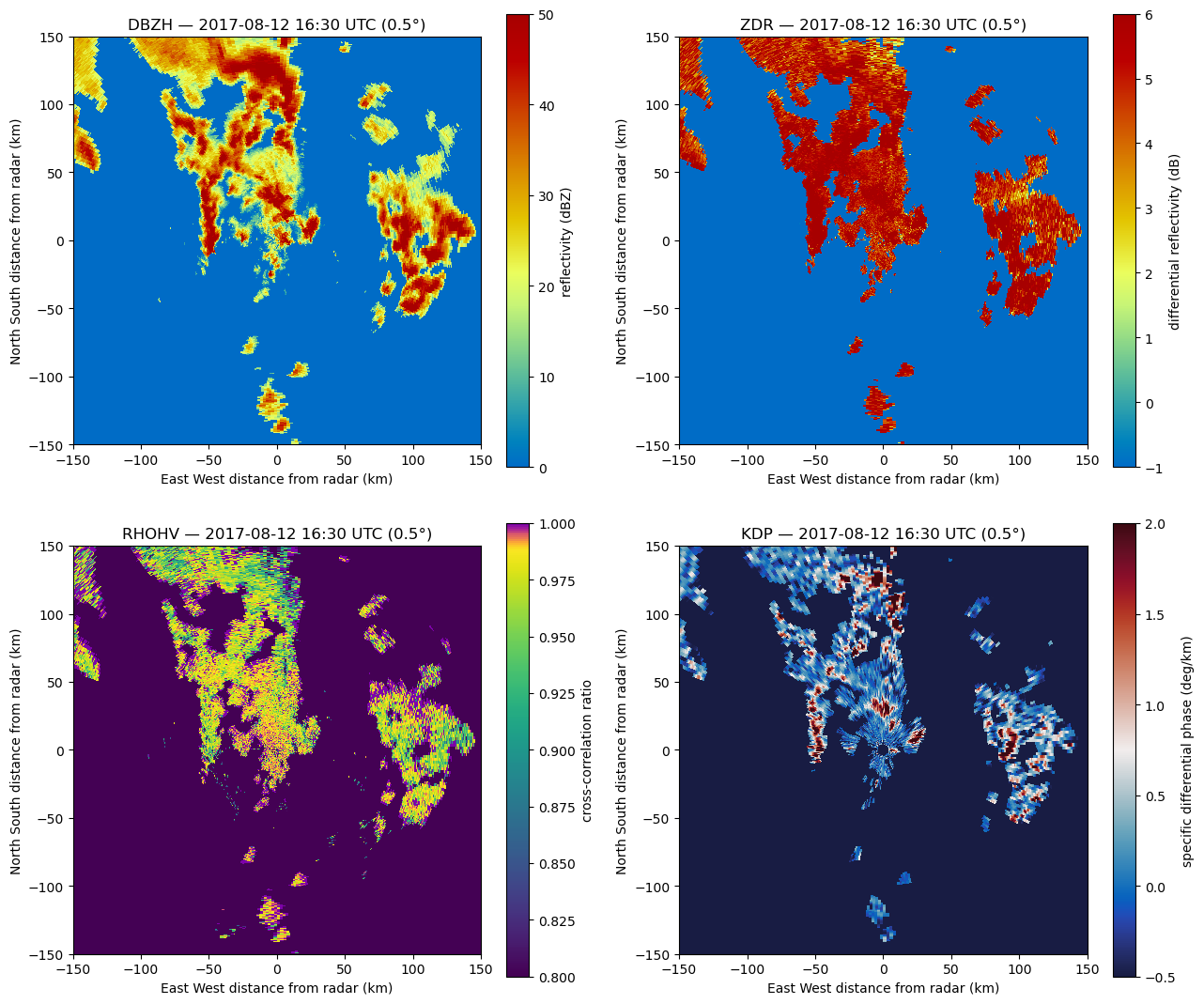

Notice that the raw $Z_{DR}$ is high almost everywhere there is echo — values of 4–6 dB across ordinary rain. Rain that heavy and uniform is not physical; this is the system offset we are about to measure.

A note on masking¶

The Leonardo processor fills below-threshold gates in two ways: a declared _FillValue of −999 (which xarray masks to NaN on read) and a “no-signal” $Z_{DR}$ floor near −8.08 dB that fills the majority of gates in any scan. Neither represents a measurement. The physical masks we apply below — a reflectivity window and a high- $\rho_{HV}$ threshold — exclude both automatically, because real light rain has neither −999 nor −8 dB $Z_{DR}$ .

Finding spherical drops¶

Small raindrops (light rain, $Z_H \approx 15$ –25 dBZ) are nearly spherical, so their intrinsic $Z_{DR}\approx 0$ dB. A high cross-correlation ratio ( $\rho_{HV} > 0.99$ ) confirms a uniform, meteorological, single-species target — excluding ground clutter, biota, melting-layer mixtures, and noise. The intersection of these conditions is our calibration population.

zdr = radar.fields["ZDR"]["data"]
rho = radar.fields["RHOHV"]["data"]
dbz = radar.fields["DBZH"]["data"]

drop_mask = (dbz >= 15) & (dbz <= 25) & (rho > 0.99) & np.isfinite(zdr)
print(f"{drop_mask.sum():,} spherical-drop gates selected across the volume")

68,386 spherical-drop gates selected across the volume

Visualise where those gates fall on the lowest sweep — they should trace the stratiform rain and avoid convective cores and clutter.

sweep0 = radar.get_slice(0)
x = radar.gate_x["data"][sweep0] / 1000.0
y = radar.gate_y["data"][sweep0] / 1000.0
m0 = drop_mask[sweep0]

fig, axes = plt.subplots(1, 3, figsize=(16.5, 5.2))
disp.plot_ppi("DBZH", sweep=0, ax=axes[0], vmin=0, vmax=50, cmap="HomeyerRainbow",
              colorbar_label="reflectivity (dBZ)", title="DBZH (0.5°)")
disp.plot_ppi("RHOHV", sweep=0, ax=axes[1], vmin=0.9, vmax=1.0, cmap="plasmidis",
              colorbar_label="cross-correlation ratio", title="RHOHV (0.5°)")
axes[2].scatter(x[~m0], y[~m0], s=0.2, c="0.85")
axes[2].scatter(x[m0], y[m0], s=0.4, c="tab:blue")
axes[2].set(title="spherical-drop gates\n(15–25 dBZ, ρHV > 0.99)",
            xlabel="x (km)", ylabel="y (km)")
for ax in axes:
    ax.set_xlim(-150, 150); ax.set_ylim(-150, 150); ax.set_aspect("equal")
fig.tight_layout()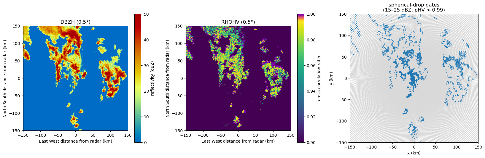

The statistical calculation¶

With the calibration population isolated, the offset is simply the median observed $Z_{DR}$ over those gates. The median is preferred over the mean because it is insensitive to the tail of larger, slightly oblate drops that survive the upper reflectivity cut.

zdr_selected = zdr[drop_mask]
zdr_offset = float(np.median(zdr_selected))

print(f"ZDR system offset : {zdr_offset:+.3f} dB")
print(f"  IQR             : {np.percentile(zdr_selected, 25):+.3f} … "
      f"{np.percentile(zdr_selected, 75):+.3f} dB")
print(f"  n gates         : {zdr_selected.size:,}")

ZDR system offset : +4.678 dB
  IQR             : +4.245 … +5.150 dB
  n gates         : 68,386

fig, ax = plt.subplots(figsize=(8.5, 5))
bins = np.linspace(-2, 8, 120)
ax.hist(zdr_selected, bins=bins, color="0.6", alpha=0.8,
        label=f"raw ZDR (median {zdr_offset:+.2f} dB)")
ax.hist(zdr_selected - zdr_offset, bins=bins, color="tab:blue", alpha=0.6,
        label="offset-corrected (median 0.00 dB)")
ax.axvline(zdr_offset, color="0.3", ls="--", lw=1.2)
ax.axvline(0, color="tab:blue", ls="--", lw=1.2)
ax.set(xlabel="ZDR (dB)", ylabel="gate count",
       title=f"ZDR in light-rain gates — Jastrebac {sel_time:%Y-%m-%d %H:%M} UTC")
ax.legend()
fig.tight_layout()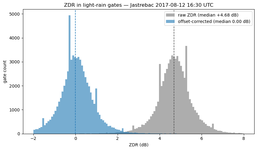

Adding the offset-corrected ZDR field¶

We subtract the offset from every sweep in the volume, working in xarray space (this keeps the correction sweep-aware and CF-clean), then re-bridge into Py-ART to plot the result.

def apply_zdr_offset(volume_tree, offset, src="ZDR", dst="ZDR_corrected"):
    """Add an offset-corrected ZDR field to every sweep of a volume DataTree."""
    out = volume_tree.copy()
    for name, node in out.children.items():
        if src in node.ds:
            ds = node.to_dataset()
            corrected = ds[src] - offset
            corrected.attrs = dict(ds[src].attrs)
            corrected.attrs["long_name"] = "Offset-corrected differential reflectivity"
            corrected.attrs["comment"] = (
                f"{src} minus {offset:.3f} dB system offset (spherical-drop method)"
            )
            out[name].ds = ds.assign({dst: corrected})
    return out


vol_corrected = apply_zdr_offset(vol, zdr_offset)
radar_corrected = Xradar(vol_corrected)
print("fields now include:", "ZDR_corrected" in radar_corrected.fields)

fields now include: True

disp_c = pyart.graph.RadarDisplay(radar_corrected)
fig, axes = plt.subplots(1, 2, figsize=(13, 5.4))
disp_c.plot_ppi("ZDR", sweep=0, ax=axes[0], vmin=-1, vmax=6, cmap="HomeyerRainbow",
                colorbar_label="ZDR (dB)", title=f"raw ZDR  (offset ≈ {zdr_offset:+.2f} dB)")
disp_c.plot_ppi("ZDR_corrected", sweep=0, ax=axes[1], vmin=-1, vmax=6, cmap="HomeyerRainbow",
                colorbar_label="ZDR (dB)", title="offset-corrected ZDR")
for ax in axes:
    ax.set_xlim(-150, 150); ax.set_ylim(-150, 150); ax.set_aspect("equal")
fig.tight_layout()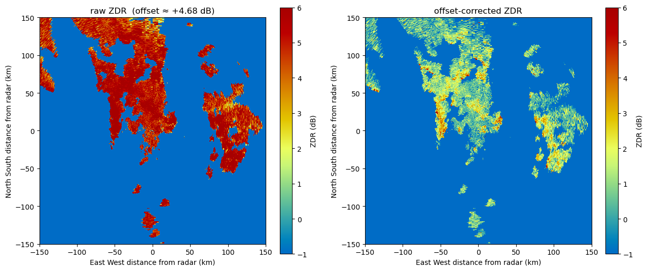

After correction, light rain sits near 0 dB and only genuinely oblate targets (heavier rain, the melting layer) stand out with positive $Z_{DR}$ — exactly what the physics predicts.

Conclusions¶

We opened a dual-pol ARCO volume with xradar, bridged it into Py-ART, isolated near-spherical drops using a reflectivity window and a $\rho_{HV}$ threshold, and took the median $Z_{DR}$ there as the system offset. Subtracting that offset restored light rain to its physical value of ~0 dB.

What’s Next¶

The offset-corrected $Z_{DR}$ can now feed quantitative retrievals — rainfall estimation, hydrometeor classification, and attenuation correction — covered in the gridding and retrieval notebooks.

Resources and References¶

Py-ART essentials links:

On $Z_{DR}$ calibration:

Bringi, V. N., & Chandrasekar, V. (2001). Polarimetric Doppler Weather Radar. Cambridge University Press.
Ryzhkov, A. V., et al. (2005). Calibration issues of dual-polarization radar measurements. J. Atmos. Oceanic Technol., 22, 1138–1155.