![]()
wradlib data quality
Overview
Within this notebook, we will cover:
Reading radar volume data into xarray based RadarVolume
Wrapping numpy-based functions to work with Xarray
Clutter detection
Beam Blockage calculation
Prerequisites
Concepts |
Importance |
Notes |
|---|---|---|
Helpful |
Basic Dataset/DataArray |
|
Helpful |
Basic Plotting |
|
Helpful |
Projections |
Time to learn: 10 minutes
Imports
import glob
import os
import cartopy
import cartopy.crs as ccrs
import cartopy.feature as cfeature
import matplotlib as mpl
import matplotlib.pyplot as plt
import numpy as np
import xarray as xr
import wradlib as wrl
Import Swiss Radar Data from CfRadial1 Volumes
We use some of the pyrad example data here. Sweeps are provided as single files, so we open each file separately and create the RadarVolume from the open Datasets.
fglob = "./data/example_pyrad/22179/MLL22179/MLL2217907250U*.nc"
flist = glob.glob(fglob)
flist.sort()
print("Files available: {}".format(len(flist)))
Files available: 20
ds = [xr.open_dataset(f, group="sweep_0", engine="cfradial1", chunks={}) for f in flist]
vol = wrl.io.RadarVolume(engine="cfradial1")
vol.extend(ds)
display(vol)
<wradlib.RadarVolume>
Dimension(s): (sweep: 20)
Elevation(s): (-0.2, 0.4, 1.0, 1.6, 2.5, 3.5, 4.5, 5.5, 6.5, 7.5, 8.5, 9.5, 11.0, 13.0, 16.0, 20.0, 25.0, 30.0, 35.0, 40.0)
sweep_number = 3
display(vol[sweep_number])
<xarray.Dataset>
Dimensions: (azimuth: 360, range: 324)
Coordinates:
time (azimuth) datetime64[ns] dask.array<chunksize=(360,), meta=np.ndarray>
* range (range) float32 250.0 ... 1.617e+05
* azimuth (azimuth) float32 0.5274 1.53 ... 359.5
elevation (azimuth) float32 dask.array<chunksize=(360,), meta=np.ndarray>
latitude float32 ...
longitude float32 ...
altitude float32 ...
Data variables: (12/14)
reflectivity (azimuth, range) float32 dask.array<chunksize=(360, 324), meta=np.ndarray>
signal_to_noise_ratio (azimuth, range) float32 dask.array<chunksize=(360, 324), meta=np.ndarray>
reflectivity_vv (azimuth, range) float32 dask.array<chunksize=(360, 324), meta=np.ndarray>
differential_reflectivity (azimuth, range) float32 dask.array<chunksize=(360, 324), meta=np.ndarray>
uncorrected_cross_correlation_ratio (azimuth, range) float32 dask.array<chunksize=(360, 324), meta=np.ndarray>
uncorrected_differential_phase (azimuth, range) float32 dask.array<chunksize=(360, 324), meta=np.ndarray>
... ...
reflectivity_hh_clut (azimuth, range) float32 dask.array<chunksize=(360, 324), meta=np.ndarray>
sweep_number int64 ...
sweep_fixed_angle float32 ...
sweep_mode |S32 ...
pulse_width (azimuth) timedelta64[ns] dask.array<chunksize=(360,), meta=np.ndarray>
nyquist_velocity (azimuth) float32 dask.array<chunksize=(360,), meta=np.ndarray>Clutter detection with Gabella
While in Switzerland, why not use the well-known clutter detection scheme by Marco Gabella et. al.
Wrap Gabella Clutter detection in Xarray apply_ufunc
The routine is implemented in wradlib in pure Numpy. Numpy based processing routines can be transformed to a first class Xarray citizen with the help of xr.apply_ufunc.
def extract_clutter(da, wsize=5, thrsnorain=0, tr1=6.0, n_p=6, tr2=1.3, rm_nans=False):
return xr.apply_ufunc(
wrl.clutter.filter_gabella,
da,
input_core_dims=[["azimuth", "range"]],
output_core_dims=[["azimuth", "range"]],
dask="parallelized",
kwargs=dict(
wsize=wsize,
thrsnorain=thrsnorain,
tr1=tr1,
n_p=n_p,
tr2=tr2,
rm_nans=rm_nans,
),
)
Calculate clutter map
Now we apply Gabella scheme and add the result to the Dataset.
swp = vol[sweep_number]
clmap = swp.reflectivity_hh_clut.pipe(
extract_clutter, wsize=5, thrsnorain=0.0, tr1=21.0, n_p=23, tr2=1.3, rm_nans=False
)
swp = swp.assign({"CMAP": clmap})
display(swp)
<xarray.Dataset>
Dimensions: (azimuth: 360, range: 324)
Coordinates:
time (azimuth) datetime64[ns] dask.array<chunksize=(360,), meta=np.ndarray>
* range (range) float32 250.0 ... 1.617e+05
* azimuth (azimuth) float32 0.5274 1.53 ... 359.5
elevation (azimuth) float32 dask.array<chunksize=(360,), meta=np.ndarray>
latitude float32 ...
longitude float32 ...
altitude float32 ...
Data variables: (12/15)
reflectivity (azimuth, range) float32 dask.array<chunksize=(360, 324), meta=np.ndarray>
signal_to_noise_ratio (azimuth, range) float32 dask.array<chunksize=(360, 324), meta=np.ndarray>
reflectivity_vv (azimuth, range) float32 dask.array<chunksize=(360, 324), meta=np.ndarray>
differential_reflectivity (azimuth, range) float32 dask.array<chunksize=(360, 324), meta=np.ndarray>
uncorrected_cross_correlation_ratio (azimuth, range) float32 dask.array<chunksize=(360, 324), meta=np.ndarray>
uncorrected_differential_phase (azimuth, range) float32 dask.array<chunksize=(360, 324), meta=np.ndarray>
... ...
sweep_number int64 ...
sweep_fixed_angle float32 ...
sweep_mode |S32 ...
pulse_width (azimuth) timedelta64[ns] dask.array<chunksize=(360,), meta=np.ndarray>
nyquist_velocity (azimuth) float32 dask.array<chunksize=(360,), meta=np.ndarray>
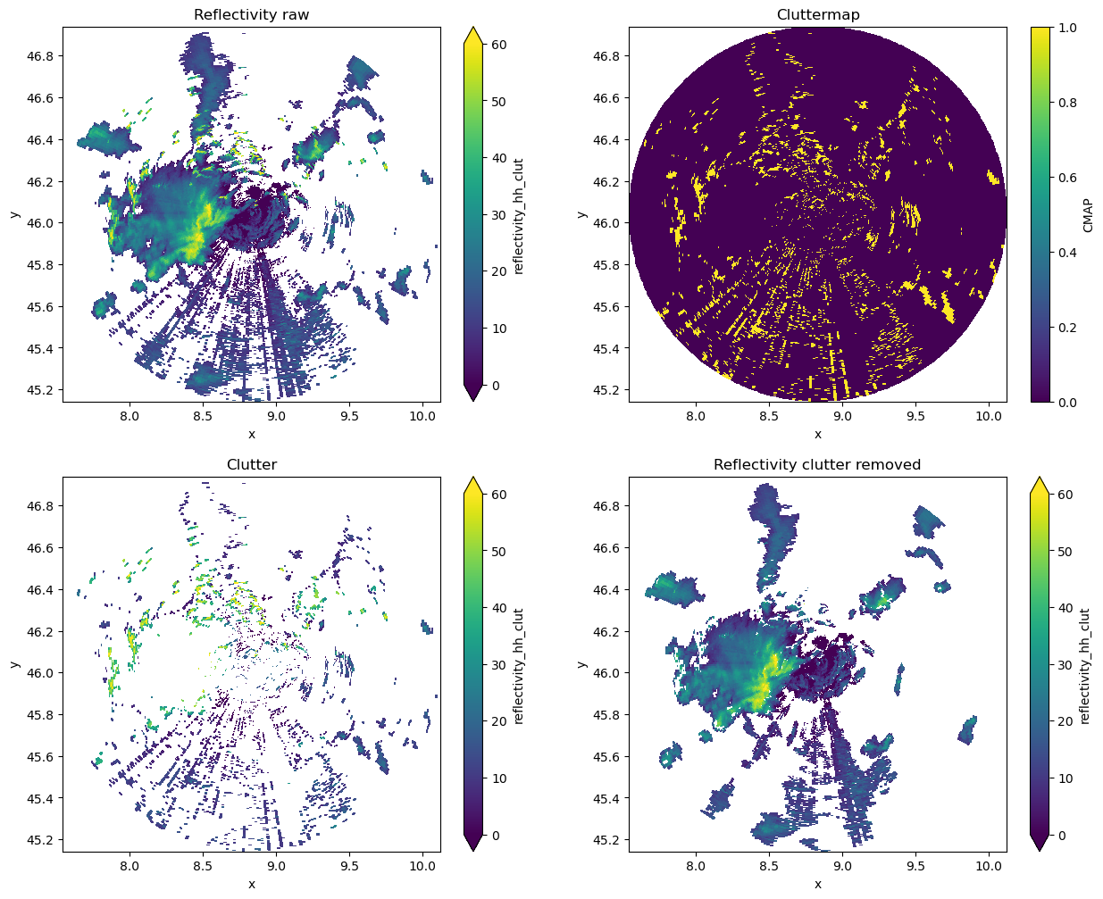
CMAP (azimuth, range) bool dask.array<chunksize=(360, 324), meta=np.ndarray>Plot Reflectivities, Clutter and Cluttermap
from osgeo import osr
wgs84 = osr.SpatialReference()
wgs84.ImportFromEPSG(4326)
0
fig = plt.figure(figsize=(15, 12))
swpx = swp.sel(range=slice(0, 100000)).pipe(wrl.georef.georeference_dataset, proj=wgs84)
ax1 = fig.add_subplot(221)
swpx.reflectivity_hh_clut.plot(x="x", y="y", ax=ax1, vmin=0, vmax=60)
ax1.set_title("Reflectivity raw")
ax2 = fig.add_subplot(222)
swpx.CMAP.plot(x="x", y="y", ax=ax2)
ax2.set_title("Cluttermap")
ax3 = fig.add_subplot(223)
swpx.reflectivity_hh_clut.where(swpx.CMAP == 1).plot(
x="x", y="y", ax=ax3, vmin=0, vmax=60
)
ax3.set_title("Clutter")
ax4 = fig.add_subplot(224)
swpx.reflectivity_hh_clut.where(swpx.CMAP < 1).plot(
x="x", y="y", ax=ax4, vmin=0, vmax=60
)
ax4.set_title("Reflectivity clutter removed")
Text(0.5, 1.0, 'Reflectivity clutter removed')
SRTM based clutter and beamblockage processing
Download needed SRTM data
For the course we already provide the needed SRTM tiles. For normal operation you would need a NASA EARTHDATA account and a connected bearer token.
The data will be loaded using GDAL machinery and transformed into an Xarray DataArray.
extent = wrl.zonalstats.get_bbox(swpx.x.values, swpx.y.values)
extent
{'left': 7.545772342625747,
'right': 10.120652596829073,
'bottom': 45.14416090772705,
'top': 46.9372157592286}
# apply fake token, data is already available
os.environ["WRADLIB_EARTHDATA_BEARER_TOKEN"] = ""
# set location of wradlib-data, where wradlib will search for any available data
os.environ["WRADLIB_DATA"] = "data/wradlib-data"
# get the tiles
dem = wrl.io.get_srtm(extent.values())
elevation = wrl.georef.read_gdal_values(dem)
coords = wrl.georef.read_gdal_coordinates(dem)
elev = xr.DataArray(
data=elevation,
dims=["y", "x"],
coords={"lat": (["y", "x"], coords[..., 1]), "lon": (["y", "x"], coords[..., 0])},
)
elev
<xarray.DataArray (y: 2401, x: 4801)>
array([[ 422, 422, 422, ..., 1846, 1798, 1745],
[ 422, 422, 422, ..., 1856, 1807, 1748],
[ 422, 422, 422, ..., 1815, 1781, 1740],
...,
[2403, 2379, 2357, ..., 14, 15, 15],
[2408, 2387, 2365, ..., 14, 15, 14],
[2428, 2411, 2397, ..., 13, 13, 13]], dtype=int16)
Coordinates:
lat (y, x) float64 47.0 47.0 47.0 47.0 47.0 ... 45.0 45.0 45.0 45.0
lon (y, x) float64 7.0 7.001 7.002 7.003 7.003 ... 11.0 11.0 11.0 11.0
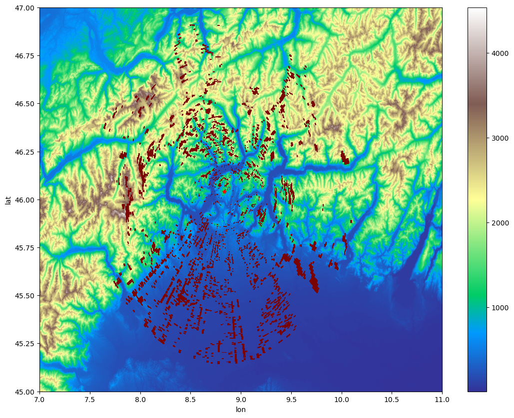
Dimensions without coordinates: y, xPlot Clutter on DEM
fig = plt.figure(figsize=(13, 10))
ax1 = fig.add_subplot(111)
swpx.CMAP.where(swpx.CMAP == 1).plot(
x="x", y="y", ax=ax1, vmin=0, vmax=1, cmap="turbo", add_colorbar=False
)
ax1.set_title("Reflectivity corr")
ax1.plot(swpx.longitude.values, swpx.latitude.values, marker="*", c="r")
elev.plot(x="lon", y="lat", ax=ax1, zorder=-2, cmap="terrain")
<matplotlib.collections.QuadMesh at 0x7f5bdb726d10>
Use hvplot for interactive zooming and panning
Often it is desirable to quickly zoom and pan in the plots. Although matplotlib has that ability, it still is quite slow. Here hvplot, a holoviews based plotting framework, can be utilized. As frontend bokeh is used.
import hvplot
import hvplot.xarray
We need to rechunk the coordinates as hvplot needs chunked variables and coords.
cl = (
swpx.CMAP.where(swpx.CMAP == 1)
.chunk(chunks={})
.hvplot.quadmesh(
x="x", y="y", cmap="Reds", width=800, height=700, clim=(0, 1), alpha=0.6
)
)
dm = elev.hvplot.quadmesh(
x="lon",
y="lat",
cmap="terrain",
width=800,
height=700,
clim=(0, 4000),
rasterize=True,
)
dm * cl
Convert DEM to spherical coordinates
sitecoords = (swpx.longitude.values, swpx.latitude.values, swpx.altitude.values)
r = swpx.range.values
az = swpx.azimuth.values
bw = 0.8
beamradius = wrl.util.half_power_radius(r, bw)
rastervalues, rastercoords, proj = wrl.georef.extract_raster_dataset(
dem, nodata=-32768.0
)
rlimits = (extent["left"], extent["bottom"], extent["right"], extent["top"])
# Clip the region inside our bounding box
ind = wrl.util.find_bbox_indices(rastercoords, rlimits)
rastercoords = rastercoords[ind[1] : ind[3], ind[0] : ind[2], ...]
rastervalues = rastervalues[ind[1] : ind[3], ind[0] : ind[2]]
polcoords = np.dstack([swpx.x.values, swpx.y.values])
# Map rastervalues to polar grid points
polarvalues = wrl.ipol.cart_to_irregular_spline(
rastercoords, rastervalues, polcoords, order=3, prefilter=False
)
Partial and Cumulative Beamblockage
PBB = wrl.qual.beam_block_frac(polarvalues, swpx.z.values, beamradius)
PBB = np.ma.masked_invalid(PBB)
print(PBB.shape)
(360, 200)
/home/jgiles/mambaforge/envs/wradlib4/lib/python3.11/site-packages/wradlib/qual.py:127: RuntimeWarning: invalid value encountered in sqrt
numer = (ya * np.sqrt(a**2 - y**2)) + (a * np.arcsin(ya)) + (np.pi * a / 2.0)
/home/jgiles/mambaforge/envs/wradlib4/lib/python3.11/site-packages/wradlib/qual.py:127: RuntimeWarning: invalid value encountered in arcsin
numer = (ya * np.sqrt(a**2 - y**2)) + (a * np.arcsin(ya)) + (np.pi * a / 2.0)
CBB = wrl.qual.cum_beam_block_frac(PBB)
print(CBB.shape)
(360, 200)
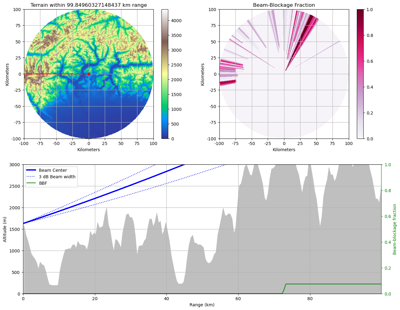
Plotting Beamblockage
# just a little helper function to style x and y axes of our maps
def annotate_map(ax, cm=None, title=""):
xticks = ax.get_xticks()
ticks = (xticks / 1000).astype(int)
ax.set_xticks(xticks)
ax.set_xticklabels(ticks)
yticks = ax.get_yticks()
ticks = (yticks / 1000).astype(int)
ax.set_yticks(yticks)
ax.set_yticklabels(ticks)
ax.set_xlabel("Kilometers")
ax.set_ylabel("Kilometers")
if not cm is None:
plt.colorbar(cm, ax=ax)
if not title == "":
ax.set_title(title)
ax.grid()
alt = swpx.z.values
fig = plt.figure(figsize=(15, 12))
# create subplots
ax1 = plt.subplot2grid((2, 2), (0, 0))
ax2 = plt.subplot2grid((2, 2), (0, 1))
ax3 = plt.subplot2grid((2, 2), (1, 0), colspan=2, rowspan=1)
# azimuth angle
angle = 270
# Plot terrain (on ax1)
ax1, dem = wrl.vis.plot_ppi(
polarvalues, ax=ax1, r=r, az=az, cmap=mpl.cm.terrain, vmin=0.0
)
ax1.plot(
[0, np.sin(np.radians(angle)) * 1e5], [0, np.cos(np.radians(angle)) * 1e5], "r-"
)
ax1.plot(sitecoords[0], sitecoords[1], "ro")
annotate_map(ax1, dem, "Terrain within {0} km range".format(np.max(r / 1000.0) + 0.1))
ax1.set_xlim(-100000, 100000)
ax1.set_ylim(-100000, 100000)
# Plot CBB (on ax2)
ax2, cbb = wrl.vis.plot_ppi(CBB, ax=ax2, r=r, az=az, cmap=mpl.cm.PuRd, vmin=0, vmax=1)
annotate_map(ax2, cbb, "Beam-Blockage Fraction")
ax2.set_xlim(-100000, 100000)
ax2.set_ylim(-100000, 100000)
# Plot single ray terrain profile on ax3
(bc,) = ax3.plot(r / 1000.0, alt[angle, :], "-b", linewidth=3, label="Beam Center")
(b3db,) = ax3.plot(
r / 1000.0,
(alt[angle, :] + beamradius),
":b",
linewidth=1.5,
label="3 dB Beam width",
)
ax3.plot(r / 1000.0, (alt[angle, :] - beamradius), ":b")
ax3.fill_between(r / 1000.0, 0.0, polarvalues[angle, :], color="0.75")
ax3.set_xlim(0.0, np.max(r / 1000.0) + 0.1)
ax3.set_ylim(0.0, 3000)
ax3.set_xlabel("Range (km)")
ax3.set_ylabel("Altitude (m)")
ax3.grid()
axb = ax3.twinx()
(bbf,) = axb.plot(r / 1000.0, CBB[angle, :], "-g", label="BBF")
axb.spines["right"].set_color("g")
axb.tick_params(axis="y", colors="g")
axb.set_ylabel("Beam-blockage fraction", c="g")
axb.set_ylim(0.0, 1.0)
axb.set_xlim(0.0, np.max(r / 1000.0) + 0.1)
legend = ax3.legend(
(bc, b3db, bbf),
("Beam Center", "3 dB Beam width", "BBF"),
loc="upper left",
fontsize=10,
)
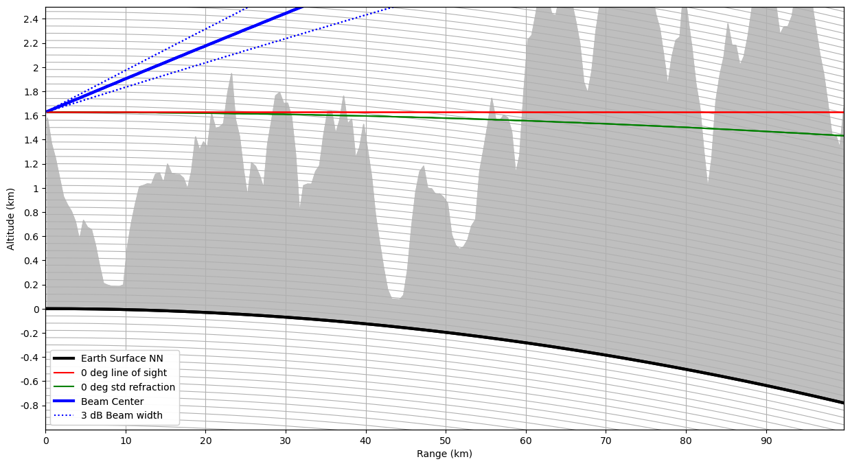
Plotting Beamblockage on Curvelinear Grid
Here you get an better impression of the actual beam progression .
def height_formatter(x, pos):
x = (x - 6370000) / 1000
fmt_str = "{:g}".format(x)
return fmt_str
def range_formatter(x, pos):
x = x / 1000.0
fmt_str = "{:g}".format(x)
return fmt_str
fig = plt.figure(figsize=(15, 8))
cgax, caax, paax = wrl.vis.create_cg(fig=fig, rot=0, scale=1)
# azimuth angle
angle = 270
# fix grid_helper
er = 6370000
gh = cgax.get_grid_helper()
gh.grid_finder.grid_locator2._nbins = 80
gh.grid_finder.grid_locator2._steps = [1, 2, 4, 5, 10]
# calculate beam_height and arc_distance for ke=1
# means line of sight
bhe = wrl.georef.bin_altitude(r, 0, sitecoords[2], re=er, ke=1.0)
ade = wrl.georef.bin_distance(r, 0, sitecoords[2], re=er, ke=1.0)
nn0 = np.zeros_like(r)
# for nice plotting we assume earth_radius = 6370000 m
ecp = nn0 + er
# theta (arc_distance sector angle)
thetap = -np.degrees(ade / er) + 90.0
# zero degree elevation with standard refraction
bh0 = wrl.georef.bin_altitude(r, 0, sitecoords[2], re=er)
# plot (ecp is earth surface normal null)
(bes,) = paax.plot(thetap, ecp, "-k", linewidth=3, label="Earth Surface NN")
(bc,) = paax.plot(thetap, ecp + alt[angle, :], "-b", linewidth=3, label="Beam Center")
(bc0r,) = paax.plot(thetap, ecp + bh0, "-g", label="0 deg Refraction")
(bc0n,) = paax.plot(thetap, ecp + bhe, "-r", label="0 deg line of sight")
(b3db,) = paax.plot(
thetap, ecp + alt[angle, :] + beamradius, ":b", label="+3 dB Beam width"
)
paax.plot(thetap, ecp + alt[angle, :] - beamradius, ":b", label="-3 dB Beam width")
# orography
paax.fill_between(thetap, ecp, ecp + polarvalues[angle, :], color="0.75")
# shape axes
cgax.set_xlim(0, np.max(ade))
cgax.set_ylim([ecp.min() - 1000, ecp.max() + 2500])
caax.grid(True, axis="x")
cgax.grid(True, axis="y")
cgax.axis["top"].toggle(all=False)
caax.yaxis.set_major_locator(
mpl.ticker.MaxNLocator(steps=[1, 2, 4, 5, 10], nbins=20, prune="both")
)
caax.xaxis.set_major_locator(mpl.ticker.MaxNLocator())
caax.yaxis.set_major_formatter(mpl.ticker.FuncFormatter(height_formatter))
caax.xaxis.set_major_formatter(mpl.ticker.FuncFormatter(range_formatter))
caax.set_xlabel("Range (km)")
caax.set_ylabel("Altitude (km)")
legend = paax.legend(
(bes, bc0n, bc0r, bc, b3db),
(
"Earth Surface NN",
"0 deg line of sight",
"0 deg std refraction",
"Beam Center",
"3 dB Beam width",
),
loc="lower left",
fontsize=10,
)
Use Clutter and Beamblockage as Quality Index
Simple masking with cumulative beam blockage and Gabella.
swpx = swpx.assign({"CBB": (["azimuth", "range"], CBB)})
# recalculate georeferencing for AEQD
swpx = swpx.pipe(wrl.georef.georeference_dataset)
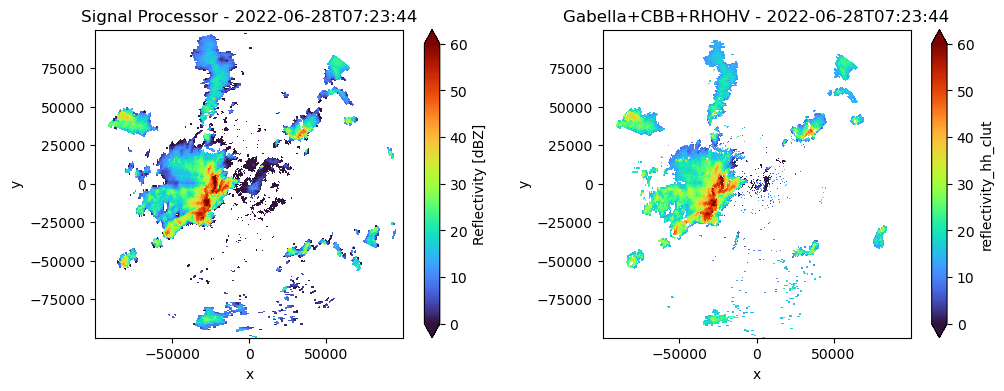
fig = plt.figure(figsize=(12, 4))
ax1 = fig.add_subplot(121)
swpx.reflectivity.plot(x="x", y="y", ax=ax1, cmap="turbo", vmin=0, vmax=60)
ax1.set_title(f"Signal Processor - {swpx.time.values.astype('M8[s]')[0]}")
ax1.set_aspect("equal")
ax2 = fig.add_subplot(122)
# CBB > 0.5, CMAP == 1, RHOHV < 0.8 is masked
swpx.where(
(swpx.CBB <= 0.5)
& (swpx.CMAP < 1.0)
& (swpx.uncorrected_cross_correlation_ratio >= 0.8)
).reflectivity_hh_clut.plot(x="x", y="y", ax=ax2, cmap="turbo", vmin=0, vmax=60)
ax2.set_title(f"Gabella+CBB+RHOHV - {swpx.time.values.astype('M8[s]')[0]}")
ax2.set_aspect("equal")
Summary
We’ve just learned how to use \(\omega radlib\)’s Gabella clutter detection for single sweeps. Wrapping numpy based functions for use with xarray.apply_ufunc has been shown. We’ve looked into digital elevation maps and beam blockage calculations.