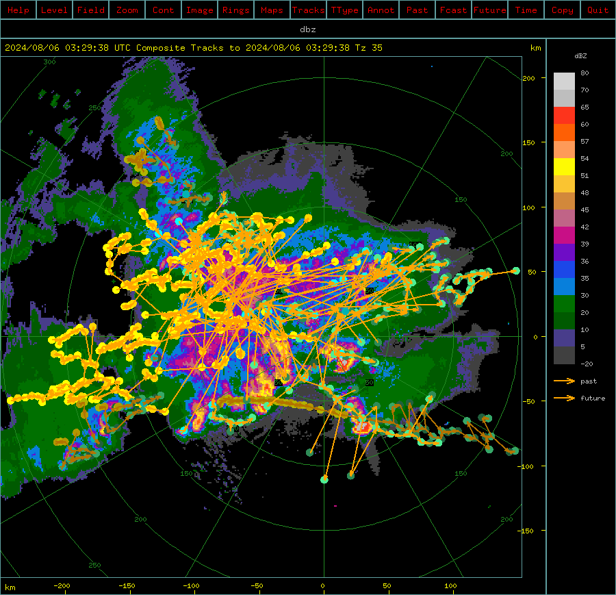
This interactive tutorial takes you through the steps of how to run the Thunderstorm Identification, Tracking, Analysis and Nowcasting (TITAN) application and analyze the output. TITAN was originally designed as an algorithm to objectively identify and track thunderstorms from weather radar data for a weather modification experiment in South Africa in the 1980s. Now, TITAN includes forecasting, storm analysis, and climatological analysis. TITAN now refers to the larger system in which the original application is one component.
TITAN is described in more detail in Dixon and Wiener (1993), and in the NSF NCAR TITAN GitHub Repo.
TITAN Background
TITAN identifies storm objects as a contiguous region of echo that exceeds a user-defined reflectivity threshold and minimum volume. Dual thresholds are used to deal with storm objects that briefly touch, but do not merge. Storm tracking is performed by looking for regions of overlap between storm objects at successive time intervals. Short term storm extrapolation forecasts are used to identify instances of storm merging and splitting. TITAN output includes storm tracks, polygons outlining the storm objects, and storm property information (e.g., volume, area, mass, precipitation flux).
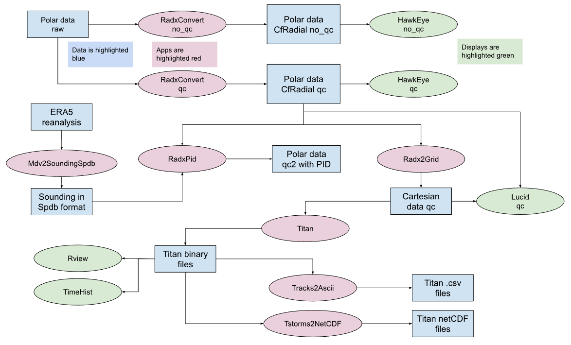
The high-level workflow for TITAN is shown in the graphic below. Key steps include quality controlling the data to remove any non-meteorological or compromised echoes and gridding the data to a Cartesian grid. Once TITAN is run and the tracks are produced, those data need to be converted into more user-friendly file types.

A more detailed workflow for TITAN that includes each step, application, and data type is shown in the graphic below.
Tutorial Overview
1. Setup
Pre-processed data and prepare parameter files
Files required to run this notebook:
Quality controlled radar data between 1600-1700 UTC.
Jastrebac is a 10 cm (S-band) Gematronik dual polarization radar in Serbia, supervised by the Republic Hydrometeorological Service of Serbia (RHMZ). This hourlong period contains areas of convection in the region.
The QC’d data is hosted on the NSF Open Storage Network (OSN) (see Data Access — Serbian Rainbow Radar for the general access pattern):
s3://nexrad-arco/lrose/cfrad/20170812/2. Output data
After the full analysis is run, the following data files should exist:
  ./data/titan/storms/20170812.th5 (TITAN binary files)
  ./data/titan/ascii/Tracks2Ascii20170812.txt (TITAN output converted by Tracks2Ascii)
1. Setup
Environment and packages
First, we import the required python packages to run this notebook. The LROSE processing can be done with the os package and shell commands.
import os
import warnings
from pathlib import Path

import fsspec

warnings.filterwarnings("ignore")
We use the same OSN access pattern shown in Data Access — Serbian Rainbow Radar:
OSN_ENDPOINT = "https://umn1.osn.mghpcc.org"
BUCKET = "nexrad-arco"
prefix = "lrose/cfrad/20170812"
1.1 Set up directories
We need to set up the required data directories. The raw radar data will be grabbed from the S3 bucket. We delete any existing files and directories specific to this tutorial to ensure we’re starting with clean directories and files.
# make overall TITAN directory and application output directory
!mkdir -p ./data/titan

# make directory for output ascii files from TITAN
!mkdir -p ./data/titan/ascii

# make directory for the raw CfRadial data pulled from OSN
!mkdir -p ./data/radar/cfrad/20170812
1.2 Set up the environment
First, we’ll set some key variables we’ll need throughout the workflow.
# Set directory variable to call LROSE
os.environ["LROSE_DIR"] = "/usr/local/lrose/bin"
1.3 Get data and convert to MDV format
We will use the data that was quality controlled in the earlier part of the day during the ERAD workshop.
TITAN requires a specialty format called MDV, which is a form of NetCDF. Since the quality controlled data are in polar coordinates, we use Radx2Grid to regrid the data to MDV. A parameter file has been provided.
!$LROSE_DIR/Radx2Grid -params ./params/Radx2Grid.params
# download the QC'd CfRadial files from OSN (anonymous read access)
fs = fsspec.filesystem(
    "s3", anon=True, client_kwargs={"endpoint_url": OSN_ENDPOINT},
)

download_dir = Path("./data/radar/cfrad/20170812")
remote_files = sorted(fs.glob(f"{BUCKET}/{prefix}/*.nc"))

for remote in remote_files:
    local = download_dir / Path(remote).name
    if not local.exists():
        fs.get(remote, str(local))
    print(f"  {local.name}")
cfrad.20170812_160007.000_to_20170812_160332.959_Jastrebac_SUR.nc
cfrad.20170812_160507.000_to_20170812_160832.999_Jastrebac_SUR.nc
cfrad.20170812_161007.000_to_20170812_161332.960_Jastrebac_SUR.nc
cfrad.20170812_161507.000_to_20170812_161833.958_Jastrebac_SUR.nc
cfrad.20170812_162007.000_to_20170812_162331.998_Jastrebac_SUR.nc
cfrad.20170812_162507.000_to_20170812_162832.958_Jastrebac_SUR.nc
cfrad.20170812_163007.000_to_20170812_163332.957_Jastrebac_SUR.nc
cfrad.20170812_163507.000_to_20170812_163832.958_Jastrebac_SUR.nc
cfrad.20170812_164007.000_to_20170812_164332.958_Jastrebac_SUR.nc
cfrad.20170812_164507.000_to_20170812_164832.959_Jastrebac_SUR.nc
cfrad.20170812_165007.000_to_20170812_165332.959_Jastrebac_SUR.nc
cfrad.20170812_165507.000_to_20170812_165831.959_Jastrebac_SUR.nc
# Grid the polar data onto a Cartesian grid
!$LROSE_DIR/Radx2Grid -params ./params/Radx2Grid.params
/usr/local/lrose/bin/Radx2Grid: /srv/conda/envs/notebook/lib/libcurl.so.4: no version information available (required by /lib/x86_64-linux-gnu/libhdf5_serial.so.103)
======================================================================
Program 'Radx2Grid'
Run-time 2026/08/22 07:08:17.
Copyright (c) 1992 - 2026
University Corporation for Atmospheric Research (UCAR)
National Center for Atmospheric Research (NCAR)
Boulder, Colorado, USA.
Redistribution and use in source and binary forms, with
or without modification, are permitted provided that the following
conditions are met:
1) Redistributions of source code must retain the above copyright
notice, this list of conditions and the following disclaimer.
2) Redistributions in binary form must reproduce the above copyright
notice, this list of conditions and the following disclaimer in the
documentation and/or other materials provided with the distribution.
3) Neither the name of UCAR, NCAR nor the names of its contributors, if
any, may be used to endorse or promote products derived from this
software without specific prior written permission.
4) If the software is modified to produce derivative works, such modified
software should be clearly marked, so as not to confuse it with the
version available from UCAR.
======================================================================
2. Run TITAN storm tracking
To start, we have provided all necessary parameters for you, so you can get a sense for the steps needed to run TITAN. We have provided basic parameters including variable names, directories, etc. Once you’ve completed the first run, you can modify a few parameters and see how the analysis changes (see Section 5).
Run the TITAN algorithm to identify and track storms.
Titan runs on the Cartesian gridded data, using the DBZ field and optionally the VEL field to compute storm rotation.
NOTE: TITAN requires a sounding to convert reflectivity data into meaningful storm metrics for the analysis. The sounding can be ingested in SPDB format or entered manually. In our case, we manually entered 10 levels retrieved from an ERA5 sounding corresponding to the radar’s location and the date and time of this case. You can verify this by inspecting the parameter files and searching for “sounding_mode = SPECIFY_SOUNDING;”, along with the manually entered array in that section.
Task #1: Run Titan on the Jastrebac data.
!$LROSE_DIR/Titan -params ./params/Titan.params -start “2017 08 12 16 00 00” -end “2017 08 12 17 00 00” -debug
# run Titan
!$LROSE_DIR/Titan -params ./params/Titan.params -start "2017 08 12 16 00 00" -end "2017 08 12 17 00 00" -debug
/usr/local/lrose/bin/Titan: /srv/conda/envs/notebook/lib/libcurl.so.4: no version information available (required by /lib/x86_64-linux-gnu/libhdf5_serial.so.103)
======================================================================
Program 'Titan'
Run-time 2026/08/22 07:09:12.
Copyright (c) 1992 - 2026
University Corporation for Atmospheric Research (UCAR)
National Center for Atmospheric Research (NCAR)
Boulder, Colorado, USA.
Redistribution and use in source and binary forms, with
or without modification, are permitted provided that the following
conditions are met:
1) Redistributions of source code must retain the above copyright
notice, this list of conditions and the following disclaimer.
2) Redistributions in binary form must reproduce the above copyright
notice, this list of conditions and the following disclaimer in the
documentation and/or other materials provided with the distribution.
3) Neither the name of UCAR, NCAR nor the names of its contributors, if
any, may be used to endorse or promote products derived from this
software without specific prior written permission.
4) If the software is modified to produce derivative works, such modified
software should be clearly marked, so as not to confuse it with the
version available from UCAR.
======================================================================
***************** ARCHIVE MODE **********************
overlapStartTime: 2017/08/12 16:00:00 UTC
startTime: 2017/08/12 16:00:00 UTC
endTime: 2017/08/12 17:00:00 UTC
*****************************************************
Read input file: ./data/radar/cart//20170812/ncf_20170812_160332.nc
========== identification ========
Scan number 0
  nstorms : 54
  Time: 2017/08/12 16:03:32
Read input file: ./data/radar/cart//20170812/ncf_20170812_160832.nc
========== identification ========
Scan number 1
  nstorms : 61
  Time: 2017/08/12 16:08:32
------------ tracking ------------
Tracking scan 0 to scan 1
  Time 1: 2017/ 8/12 16: 3:32, nstorms 54
  Time 2: 2017/ 8/12 16: 8:32, nstorms 61
  Dtime (secs) : 300
Read input file: ./data/radar/cart//20170812/ncf_20170812_161332.nc
========== identification ========
Scan number 2
  nstorms : 63
  Time: 2017/08/12 16:13:32
------------ tracking ------------
Tracking scan 1 to scan 2
  Time 1: 2017/ 8/12 16: 8:32, nstorms 61
  Time 2: 2017/ 8/12 16:13:32, nstorms 63
  Dtime (secs) : 300
Read input file: ./data/radar/cart//20170812/ncf_20170812_161833.nc
========== identification ========
Scan number 3
  nstorms : 59
  Time: 2017/08/12 16:18:33
------------ tracking ------------
Tracking scan 2 to scan 3
  Time 1: 2017/ 8/12 16:13:32, nstorms 63
  Time 2: 2017/ 8/12 16:18:33, nstorms 59
  Dtime (secs) : 301
Read input file: ./data/radar/cart//20170812/ncf_20170812_162331.nc
========== identification ========
Scan number 4
  nstorms : 68
  Time: 2017/08/12 16:23:31
------------ tracking ------------
Tracking scan 3 to scan 4
  Time 1: 2017/ 8/12 16:18:33, nstorms 59
  Time 2: 2017/ 8/12 16:23:31, nstorms 68
  Dtime (secs) : 298
Read input file: ./data/radar/cart//20170812/ncf_20170812_162832.nc
========== identification ========
Scan number 5
  nstorms : 61
  Time: 2017/08/12 16:28:32
------------ tracking ------------
Tracking scan 4 to scan 5
  Time 1: 2017/ 8/12 16:23:31, nstorms 68
  Time 2: 2017/ 8/12 16:28:32, nstorms 61
  Dtime (secs) : 301
Read input file: ./data/radar/cart//20170812/ncf_20170812_163332.nc
========== identification ========
Scan number 6
  nstorms : 56
  Time: 2017/08/12 16:33:32
------------ tracking ------------
Tracking scan 5 to scan 6
  Time 1: 2017/ 8/12 16:28:32, nstorms 61
  Time 2: 2017/ 8/12 16:33:32, nstorms 56
  Dtime (secs) : 300
Read input file: ./data/radar/cart//20170812/ncf_20170812_163832.nc
========== identification ========
Scan number 7
  nstorms : 57
  Time: 2017/08/12 16:38:32
------------ tracking ------------
Tracking scan 6 to scan 7
  Time 1: 2017/ 8/12 16:33:32, nstorms 56
  Time 2: 2017/ 8/12 16:38:32, nstorms 57
  Dtime (secs) : 300
Read input file: ./data/radar/cart//20170812/ncf_20170812_164332.nc
========== identification ========
Scan number 8
  nstorms : 54
  Time: 2017/08/12 16:43:32
------------ tracking ------------
Tracking scan 7 to scan 8
  Time 1: 2017/ 8/12 16:38:32, nstorms 57
  Time 2: 2017/ 8/12 16:43:32, nstorms 54
  Dtime (secs) : 300
Read input file: ./data/radar/cart//20170812/ncf_20170812_164832.nc
========== identification ========
Scan number 9
  nstorms : 54
  Time: 2017/08/12 16:48:32
------------ tracking ------------
Tracking scan 8 to scan 9
  Time 1: 2017/ 8/12 16:43:32, nstorms 54
  Time 2: 2017/ 8/12 16:48:32, nstorms 54
  Dtime (secs) : 300
Read input file: ./data/radar/cart//20170812/ncf_20170812_165332.nc
========== identification ========
Scan number 10
  nstorms : 54
  Time: 2017/08/12 16:53:32
------------ tracking ------------
Tracking scan 9 to scan 10
  Time 1: 2017/ 8/12 16:48:32, nstorms 54
  Time 2: 2017/ 8/12 16:53:32, nstorms 54
  Dtime (secs) : 300
Read input file: ./data/radar/cart//20170812/ncf_20170812_165831.nc
========== identification ========
Scan number 11
  nstorms : 53
  Time: 2017/08/12 16:58:31
------------ tracking ------------
Tracking scan 10 to scan 11
  Time 1: 2017/ 8/12 16:53:32, nstorms 54
  Time 2: 2017/ 8/12 16:58:31, nstorms 53
  Dtime (secs) : 299
3. Convert TITAN binary output to readable format
The TITAN output is in a binary format. In order to read the data, we first convert the TITAN output to an ASCII file.
Task #2: Convert Titan binary output to ASCII.
!$LROSE_DIR/Tracks2Ascii -params ./params/Tracks2Ascii.params -f ./data/titan/storms/20170812.th5 > ./data/titan/ascii/Tracks2Ascii20170812.txt -debug
!$LROSE_DIR/Tracks2Ascii -params ./params/Tracks2Ascii.params -f ./data/titan/storms/20170812.th5 > ./data/titan/ascii/Tracks2Ascii20170812.txt -debug/usr/local/lrose/bin/Tracks2Ascii: /srv/conda/envs/notebook/lib/libcurl.so.4: no version information available (required by /lib/x86_64-linux-gnu/libhdf5_serial.so.103)
======================================================================
Program 'Tracks2Ascii'
Run-time 2026/08/22 07:09:14.
Copyright (c) 1992 - 2026
University Corporation for Atmospheric Research (UCAR)
National Center for Atmospheric Research (NCAR)
Boulder, Colorado, USA.
Redistribution and use in source and binary forms, with
or without modification, are permitted provided that the following
conditions are met:
1) Redistributions of source code must retain the above copyright
notice, this list of conditions and the following disclaimer.
2) Redistributions in binary form must reproduce the above copyright
notice, this list of conditions and the following disclaimer in the
documentation and/or other materials provided with the distribution.
3) Neither the name of UCAR, NCAR nor the names of its contributors, if
any, may be used to endorse or promote products derived from this
software without specific prior written permission.
4) If the software is modified to produce derivative works, such modified
software should be clearly marked, so as not to confuse it with the
version available from UCAR.
======================================================================
Processing track file ./data/titan/storms/20170812.th5
4. Investigate Output
We’ll load the necessary Python packages and plot some of the TITAN output now.
# Import Python packages
import pandas as pd
import numpy as np
import matplotlib.pyplot as plt
import seaborn as sns
import matplotlib.dates as mdates
import cartopy.crs as ccrs
import cartopy.feature as cfeature
from shapely.geometry import Polygon
from netCDF4 import num2date
import netCDF4 as nc
# set the path for the ASCII file
file = "./data/titan/ascii/Tracks2Ascii20170812.txt"4.1 Read the ASCII file into a pandas dataframe
Open text file and adjust columns names in order to import to a pandas dataframe. Since the text file has irregular delimiters, we need to add some extra steps.
##open file and extract column names
f = open(file)
lines = f.readlines()
f.close()

label_line_index = None

for i, line in enumerate(lines):
    if 'labels' in line:
        label_line_index = i
        break
labels = lines[label_line_index].split(":", 1)[1].strip().split(",")
#the data lines are the ones that do not start with #
data_lines = [line.strip() for line in lines if not line.startswith("#")]The file last three rows are labeled “parents”, “children”, “nPolySidesPolygonRays*72”.
Parents and children columns refer to identifiers based on storm merging and splitting processes. The Polygon column shows the values for the lines from the polygon centroid to each vertex, in km. There are 72 values because each line is separated 5 deg (72*5 =360).
With that information and the “envelope_centroid” column, we can retrieve the cells envelopes at each timestep.
rows = []
for line in data_lines:
    parts = line.split()

    try:
        # Try parsing the polygon count value (always right before 72 values)
        poly_count_index = -73  # 72 floats + 1 count (the column starts with the numnber 72, which is not part of the values)

        # Parents and children may be missing
        parent_str = parts[poly_count_index - 2]
        child_str = parts[poly_count_index - 1]

        # Handle missing values marked as "-"
        parents = int(parent_str) if parent_str != '-' else np.nan
        children = int(child_str) if child_str != '-' else np.nan

        # Polygon values: skip the count, get the next 72 values
        polygon_values = list(map(float, parts[poly_count_index + 1:]))

        # Fixed columns
        fixed_cols = parts[:poly_count_index - 2]

        # Combine into one row
        row = fixed_cols + [parents, children, polygon_values]
        rows.append(row)
    except Exception as e:
        continue
# Final columns: fixed + 3 custom ones
final_labels = labels[:len(rows[0]) - 3] + ['parents', 'children', 'nPolySidesPolygonRays']
# Create DataFrame
df = pd.DataFrame(rows, columns=final_labels)
# Convert date and time columns to datetime
df['date_utc'] = pd.to_datetime(
df['Year'].astype(str) + '-' + df['Month'].astype(str).str.zfill(2) + '-' +
df['Day'].astype(str).str.zfill(2) + ' ' + df['Hour'].astype(str).str.zfill(2) + ':' +
df['Min'].astype(str).str.zfill(2) + ':' + df['Sec'].astype(str).str.zfill(2),
format='%Y-%m-%d %H:%M:%S', utc=True
)
# Print df
print(df) NSimpleTracks ComplexNum SimpleNum Year Month Day Hour Min Sec \
0 1 0 0 2017 08 12 16 03 32
1 1 0 0 2017 08 12 16 08 32
2 1 0 0 2017 08 12 16 13 32
3 1 0 0 2017 08 12 16 18 33
4 1 0 0 2017 08 12 16 23 31
.. ... ... ... ... ... .. ... .. ..
417 1 232 232 2017 08 12 16 53 32
418 1 232 232 2017 08 12 16 58 31
419 1 235 235 2017 08 12 16 43 32
420 1 235 235 2017 08 12 16 48 32
421 1 235 235 2017 08 12 16 53 32
dBZThreshold ... HailFOKRCat0-4 HailWaldvogelProb HailMassAloft(ktons) \
0 35 ... 2 0 0
1 35 ... 2 0 0
2 35 ... 2 0 0
3 35 ... 0 0 0
4 35 ... 0 0 0
.. ... ... ... ... ...
417 35 ... 2 0.6 0.456526
418 35 ... 2 1 2.06314
419 35 ... 0 0 0
420 35 ... 0 0 0
421 35 ... 0 0 0
HailVihm(kg/m2) ReflCentroidRange(km) ReflCentroidAzimuth(deg) parents \
0 0.105039 100.733 -167.624 NaN
1 0.13675 97.7179 -167.204 NaN
2 0.163864 94.5912 -166.89 NaN
3 0.109136 91.2012 -166.57 NaN
4 0 87.5572 -166.501 NaN
.. ... ... ... ...
417 0.45598 146.249 18.9528 NaN
418 0.777891 148.111 17.8519 NaN
419 0 184.877 -29.3073 NaN
420 0 186.28 -28.5815 NaN
421 0 187.939 -27.988 NaN
children nPolySidesPolygonRays \
0 NaN [2.3, 2.3, 2.3, 2.4, 2.4, 2.5, 2.6, 2.8, 3.0, ...
1 NaN [1.8, 1.8, 2.9, 2.9, 3.0, 3.1, 3.2, 3.4, 3.7, ...
2 NaN [1.5, 1.5, 1.6, 1.6, 1.6, 1.7, 5.2, 5.5, 5.1, ...
3 NaN [2.9, 2.9, 2.9, 3.0, 3.0, 3.1, 3.3, 3.5, 3.7, ...
4 NaN [2.3, 2.3, 2.3, 2.4, 2.4, 2.5, 2.7, 2.8, 3.0, ...
.. ... ...
417 NaN [6.5, 6.5, 6.6, 6.7, 6.9, 6.1, 6.3, 6.7, 7.1, ...
418 NaN [6.7, 6.7, 6.8, 6.9, 7.1, 7.3, 7.7, 8.1, 8.7, ...
419 NaN [0.8, 0.8, 0.8, 1.8, 1.9, 4.2, 4.4, 4.6, 4.9, ...
420 NaN [0.5, 0.5, 0.5, 0.5, 1.6, 1.7, 1.7, 1.8, 2.0, ...
421 NaN [2.0, 1.0, 1.0, 1.0, 1.1, 1.1, 1.2, 1.2, 1.3, ...
date_utc
0 2017-08-12 16:03:32+00:00
1 2017-08-12 16:08:32+00:00
2 2017-08-12 16:13:32+00:00
3 2017-08-12 16:18:33+00:00
4 2017-08-12 16:23:31+00:00
.. ...
417 2017-08-12 16:53:32+00:00
418 2017-08-12 16:58:31+00:00
419 2017-08-12 16:43:32+00:00
420 2017-08-12 16:48:32+00:00
421 2017-08-12 16:53:32+00:00
[422 rows x 80 columns]
Let’s explore the TITAN output now!
4.2 Examine the number of identified individual storms per complex
How does TITAN work?
TITAN identifies individual radar cells within each radar volume based on reflectivity and volume thresholds. It then tracks these cells over time using a combination and optimization scheme, along with geometric logic to handle storm splitting and merging. In this example, we set the minimum reflectivity threshold to 35 dBZ, shown in the ‘dBZThreshold’ column. This threshold defines the minimum reflectivity value for an entity to be classified as a ‘cell’.
What is the TITAN output?
TITAN outputs cell features at each tracking timestep and identifies individual cells within larger systems based on their interaction with neighboring cells. As a result, each cell in the TITAN output ASCII file is assigned two identifiers: a “SimpleNum” and a “ComplexNum”. For example, when tracking a multicell system, each individual cell within it will have a distinct “SimpleNum,” but all cells belonging to that same system will share a common “ComplexNum.”
Let’s inspect our case now! How many Complexes can we identify? Which one contains more tracks (e.g., single cell tracks, and split/merge processes)?
# Count number of unique SimpleNum per ComplexNum
simple_counts = df.groupby('ComplexNum')['SimpleNum'].nunique().reset_index(name='NumSimple')

# Sort (optional, for better visuals)
#simple_counts = simple_counts.sort_values(by='NumSimple', ascending=False)

# Plot 1
plt.figure(figsize=(10, 8))
sns.barplot(y='ComplexNum', x='NumSimple', data=simple_counts, palette='Set3')
plt.title('Number of SimpleNum per ComplexNum', fontsize=16)
plt.xlabel('Count of Unique SimpleNum ID', fontsize=14)
plt.ylabel('ComplexNum ID', fontsize=14)
plt.xticks(fontsize=12)
plt.yticks(fontsize=12)
plt.tight_layout()
plt.grid(axis='x')
plt.show()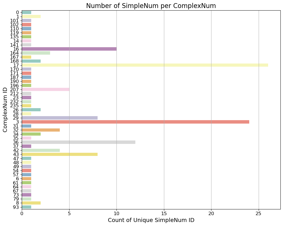
4.3 Explore a single complex
Let’s now explore one of the Complex tracks. In this case, it makes sense to choose ComplexNum = 17, which contains more than 25 tracked individual storms.
In our case, we will plot the Maximum Reflectivity ('MaxDBZ(dBZ)') for the entire life cycle of this complex system. Each individual storm is plotted in a different color (see the hue='SimpleNum' parameter in the plot).
You can play and choose another attribute (e.g., Echo Top, Vil) from the ASCII file, and see how the attributes vary.
# feel free to modify this variable based on the plot above to see what other complex tracks look like
complexnum = "17"
# Filter dataframe for the chosen ComplexNum and sort by time
df0 = df[df['ComplexNum'] == complexnum].copy()
df0 = df0.sort_values('date_utc')
df0['MaxDBZ(dBZ)'] = pd.to_numeric(df0['MaxDBZ(dBZ)'], errors='coerce')
df0['date_utc'] = pd.to_datetime(df0['date_utc'], errors='coerce', utc=True)
# Plot
y_min = 30
y_max = 70
y_ticks = np.arange(y_min, y_max + 1, 5)
plt.figure(figsize=(12, 6))
sns.set_style("whitegrid")
sns.lineplot(data=df0, x='date_utc', y='MaxDBZ(dBZ)', hue='SimpleNum', palette='gist_ncar')
plt.ylim(y_min, y_max)
plt.yticks(y_ticks,fontsize=12)
plt.gca().xaxis.set_major_formatter(mdates.DateFormatter('%H:%M'))
plt.xticks(fontsize=12)
plt.title('MaxDBZ over Time for ComplexNum = 0', fontsize=16)
plt.xlabel('Time (UTC)', fontsize=14)
plt.ylabel('MaxDBZ (dBZ)',fontsize=14)
# Remove legend
plt.legend([], [], frameon=False)
plt.tight_layout()
plt.show()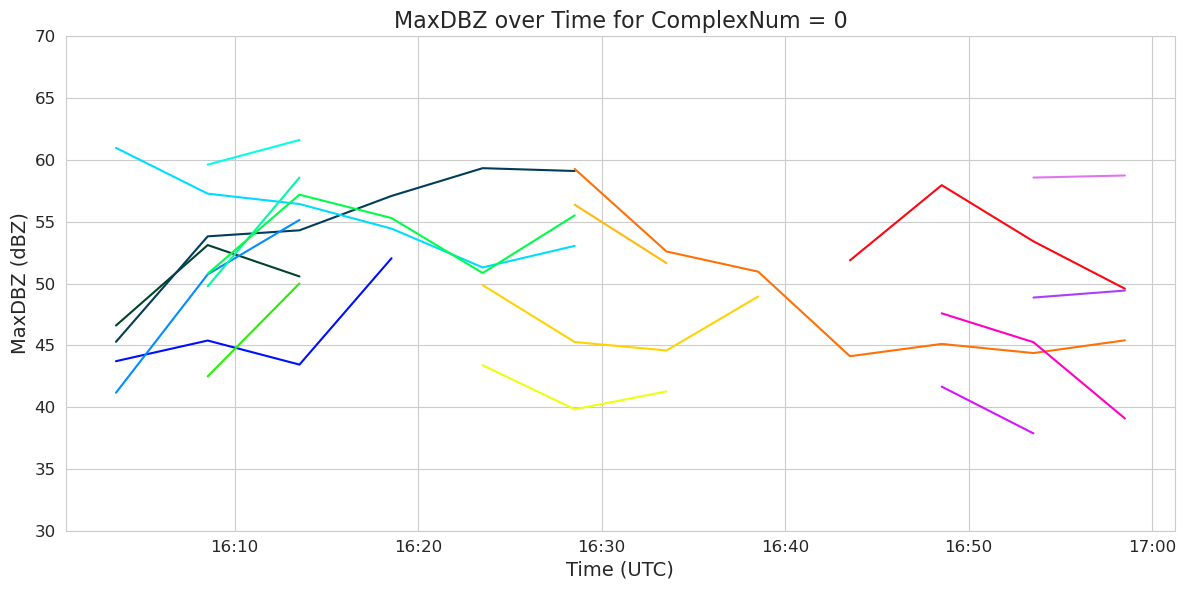
Now we can also plot the centroids of each tracked cell, in a Cartopy map, and add circles around the centroid based on how big the cell volume is in each timestep. We will also show the different cells (‘SimpleNum’) in different colors.
df0 = df0.sort_values(['SimpleNum', 'date_utc'])

# Convert lat/lon columns to numeric, coercing errors to NaN
df0['VolCentroidLat(deg)'] = pd.to_numeric(df0['VolCentroidLat(deg)'], errors='coerce')
df0['VolCentroidLon(deg)'] = pd.to_numeric(df0['VolCentroidLon(deg)'], errors='coerce')

# Set up map plot
plt.figure(figsize=(14, 10))
ax = plt.axes(projection=ccrs.PlateCarree())
ax.coastlines(resolution='10m')
ax.add_feature(cfeature.BORDERS, linestyle=':')
gl = ax.gridlines(draw_labels=True, dms=True, x_inline=False, y_inline=False)
gl.top_labels = False
gl.right_labels = False
gl.xlabel_style = {'size': 14}
gl.ylabel_style = {'size': 14}

# Force SimpleNum to categorical (string) for consistent labeling
df0['SimpleNum'] = df0['SimpleNum'].astype(str)

# Unique SimpleNum and colors
simple_nums = df0['SimpleNum'].unique()
palette = sns.color_palette("gist_ncar", n_colors=len(simple_nums))
df0['Volume(km3)'] = pd.to_numeric(df0['Volume(km3)'], errors='coerce').fillna(0)

for i, simple_num in enumerate(simple_nums):
    track = df0[df0['SimpleNum'] == simple_num].copy()
    lat = track['VolCentroidLat(deg)']
    lon = track['VolCentroidLon(deg)']
    vol = pd.to_numeric(track['Volume(km3)'], errors='coerce').fillna(0)
    sizes = np.log10(vol + 1) * 200

    ax.plot(lon, lat, marker='o', linestyle='-', color=palette[i], alpha=0.7,
             label=simple_num, transform=ccrs.PlateCarree())
    ax.scatter(lon, lat, s=sizes, color=palette[i], alpha=0.5,
               transform=ccrs.PlateCarree(), edgecolor='k', linewidth=0.5)

    # Add time labels next to each centroid
    for lo, la, t in zip(lon, lat, track['date_utc']):
        if pd.notna(lo) and pd.notna(la) and pd.notna(t):
            ax.text(lo + 0.02, la + 0.02, t.strftime('%H:%M'),
                    fontsize=8, color=palette[i], transform=ccrs.PlateCarree(),
                    ha='left', va='bottom')

ax.legend(title='SimpleNum', bbox_to_anchor=(1.02, 1), loc='upper left', fontsize=10)
plt.yticks(fontsize=12)
plt.xticks(fontsize=12)
plt.title('Tracks for ComplexNum = '+complexnum, fontsize=16)
plt.tight_layout()
plt.show()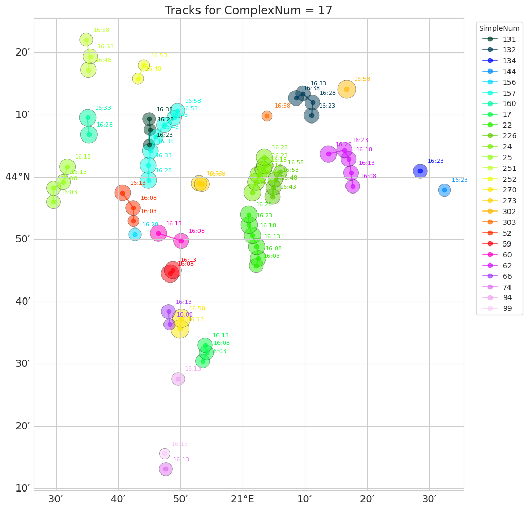
4.4 Examine radar data and storm polygons together
Now let’s plot the cartesian radar data at 16:13 UTC and overlap the polygons of the storms that we have identified with Titan.
TIME_IDX = 0

FILEPATH = "./data/radar/cart/20170812/ncf_20170812_161332.nc"   # <-- set your file path here
FIELD_NAME = "DBZ"

with nc.Dataset(FILEPATH, "r") as ds:
    x = ds.variables["lon0"][:]
    y = ds.variables["lat0"][:]

    var = ds.variables[FIELD_NAME]
    data_3d = var[TIME_IDX, :, :, :]  # all z-levels: shape (z0, y0, x0)

    fill_value = getattr(var, "_FillValue", None)
    if fill_value is not None:
        data_3d = np.ma.masked_equal(data_3d, fill_value)
    data_3d = np.ma.masked_invalid(data_3d)

    # Retrieve Max reflectivity in column ( max across the z-axis )
    data = data_3d.max(axis=0)  # shape (y0, x0)

    vmin = getattr(var, "min_value", -10.0)
    vmax = getattr(var, "max_value", 70.0)
    units = getattr(var, "units", FIELD_NAME)

    time_var = ds.variables["time"]
    raw_time = num2date(time_var[TIME_IDX], units=time_var.units,
                         calendar=getattr(time_var, "calendar", "standard"))
    plot_time = pd.Timestamp(raw_time.isoformat())


# Handle tz-naive/aware consistently
if plot_time.tz is None:
    plot_time = plot_time.tz_localize("UTC")
else:
    plot_time = plot_time.tz_convert("UTC")

plot_time_min = plot_time.floor("min")
print("Plotting field for time:", plot_time_min)
print(f"Max reflectivity in column — min/max over field: {data.min():.2f} / {data.max():.2f}")

# Correct dtypes for Dataframe
df['date_utc'] = pd.to_datetime(df['date_utc'], utc=True)
df['EnvelopeCentroidLon(deg)'] = pd.to_numeric(df['EnvelopeCentroidLon(deg)'], errors='coerce')
df['EnvelopeCentroidLat(deg)'] = pd.to_numeric(df['EnvelopeCentroidLat(deg)'], errors='coerce')

# Filter dataframe: match to the minute, within radar domain
lon_min, lon_max = float(x.min()), float(x.max())
lat_min, lat_max = float(y.min()), float(y.max())

df_match = df[
    (df['date_utc'].dt.floor("min") == plot_time_min) &
    (df['EnvelopeCentroidLon(deg)'] >= lon_min) &
    (df['EnvelopeCentroidLon(deg)'] <= lon_max) &
    (df['EnvelopeCentroidLat(deg)'] >= lat_min) &
    (df['EnvelopeCentroidLat(deg)'] <= lat_max)
]

# plot
fig, ax = plt.subplots(figsize=(12, 12), subplot_kw={'projection': ccrs.PlateCarree()})

ax.set_extent([lon_min, lon_max, lat_min, lat_max], crs=ccrs.PlateCarree())

mesh = ax.pcolormesh(
    x, y, data,
    transform=ccrs.PlateCarree(),
    shading="auto", cmap="turbo",
    vmin=vmin, vmax=vmax,
    zorder=1,
)
plt.colorbar(mesh, ax=ax, label=units, shrink=0.7)

ax.coastlines(zorder=3)

gl = ax.gridlines(draw_labels=True, dms=True, x_inline=False, y_inline=False)
gl.top_labels = False
gl.right_labels = False
gl.xlabel_style = {'size': 14}
gl.ylabel_style = {'size': 14}

#  Overlay only the matching polygons
palette = sns.color_palette("gist_ncar", n_colors=max(len(df_match), 1))

for i, (idx, row) in enumerate(df_match.iterrows()):
    lat_centroid = float(row['EnvelopeCentroidLat(deg)'])
    lon_centroid = float(row['EnvelopeCentroidLon(deg)'])
    rays = row['nPolySidesPolygonRays']

    if not rays or len(rays) == 0:
        continue

    angles = np.deg2rad(np.arange(0, 360, 5))
    rays = np.array(rays, dtype=float)

    ray_x = rays * np.cos(angles)
    ray_y = rays * np.sin(angles)
    lat_vertices = lat_centroid + ray_y / 111
    lon_vertices = lon_centroid + ray_x / (111 * np.cos(np.deg2rad(lat_centroid)))
    polygon_points = list(zip(lon_vertices, lat_vertices))

    poly = Polygon(polygon_points)
    ax.add_geometries([poly], crs=ccrs.PlateCarree(),
                       edgecolor='black', facecolor='none', linewidth=1.5,
                       zorder=4)

    ax.plot(lon_centroid, lat_centroid, marker='o', color='black', markersize=3,
             transform=ccrs.PlateCarree(), zorder=5)

plt.title(f"Max Reflectivity in Column with Track Polygons — {plot_time_min}", fontsize=16)
plt.tight_layout()
plt.show()
Plotting field for time: 2017-08-12 16:13:00+00:00
Max reflectivity in column — min/max over field: -1.22 / 68.21
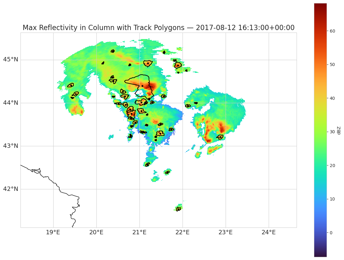
As you can see, some reflectivity regions have not been identified with polygons, while some polygons may be too large for the regions they represent. TITAN can track storms based on a variety of parameters, and users can tune these parameters to tailor which systems and storms are identified. You can explore that in the following section.
5. Explore how the storm track analysis is impacted by key parameters
Now that you’ve successfully run TITAN, we invite you to explore how parameter selection affects the final analysis. Here, we’ll focus on three groups of parameters.
5.1 Reflectivity threshold
A key parameter for TITAN is the minimum reflectivity value considered for storm identification: low_dbz_threshold. Storms are defined as regions with reflectivity values in excess of this value.
The default value for low_dbz_threshold in TITAN is 35 dBZ, but this may need to change based on the air mass, storm type, etc.
Values to consider testing for low_dbz_threshold:
30 dBZ
40 dBZ
45 dBZ
5.2 Tracking variable
Titan offers two options for the storm tracking variable: 1) the 3-D reflectivity field (default) and 2) the column maximum reflectivity. This option is set in the variable use_column_max_dbz, where FALSE (default) tracks the 3-D reflectivity field and TRUE tracks the column maximum reflectivity.
Note, if use_column_max_dbz = TRUE, then the user must set the height range over which the maximum reflectivity is calculated using the following parameters: column_min_ht_km, and column_max_ht_km.
Consider testing:
use_column_max_dbz = TRUE
5.3 Storm size parameters
Users have control over the storm sizes that TITAN tracks. You can test and change the limits to the storm base and top height (km), as well as the storm size. In terms of storm size, if the data are 2D (depending on the tracking variable), the units are km^2; if the data are 3D, the units are km^3.
Consider testing with other values:
min_storm_size
maz_storm_size
base_threshold
top_threshold
5.4 Setting up alternate parameter files and directories
We strongly recommend creating new parameter files and output directories so that you retain all examples from today.
To create a new parameter file with existing parameters, run a variation of the following command, updating the output file name at the end. The parameter file can be opened through the JupyterHub interface as text files or with your favorite Unix editor (e.g., vi, vim) on a terminal.
!$LROSE_DIR/Titan -params ./params/Titan.params -print_params > ./params/Titan.params.new
To update the output directories, you can take advantage of the -odir flag for TITAN and redirect the output of Tracks2Ascii. To update the location of the TITAN binary files for Tracks2Ascii, just update the path after the -f flag. Note the three instances of the “_new” suffix below, but feel free to rename as you prefer.
!$LROSE_DIR/Titan -params ./params/Titan.params.new -odir ./data/titan/storms_new -start “2017 08 12 16 00 00” -end “2017 08 12 17 00 00” -debug
!$LROSE_DIR/Tracks2Ascii -params ./params/Tracks2Ascii.params -f ./data/titan/storms_new/20170812.th5 > ./data/titan/ascii_new/Tracks2Ascii20170812.txt -debug
When you copy the plotting code from above, you’ll need to update the ASCII file path. Based on the number of storms associated with each complex, you may need to pick a different complexnum.
# file = "./data/titan/ascii_new/Tracks2Ascii20170812.txt"
# complexnum = "17" # change to the appropriate number- Dixon, M., & Wiener, G. (1993). TITAN: Thunderstorm Identification, Tracking, Analysis, and Nowcasting—A Radar-based Methodology. Journal of Atmospheric and Oceanic Technology, 10(6), 785–797. https://doi.org/10.1175/1520-0426(1993)010<;0785:ttitaa>2.0.co;2