Stratiform Case 2014¶

import cmweather
import numpy as np
import wradlib as wrl
import matplotlib.pyplot as plt
import xarray as xr
import xradar as xd
import fsspec
import icechunk
import holoviews as hv
import hvplot
import hvplot.xarray
import pyproj
import rioxarray
import warnings
warnings.filterwarnings("ignore", category=RuntimeWarning)
warnings.filterwarnings("ignore", category=FutureWarning)

Claim Data¶

We use the ARCO data provided in Data Access — Serbian Rainbow Radar. Please refer to this notebook for details of access.

OSN_ENDPOINT = "https://umn1.osn.mghpcc.org"
BUCKET = "nexrad-arco"

# prefix = "Fgora"  # single-pol, 12 sweeps × 360 az × 250 range, 2014 + 2017 + 2026
prefix = "jastrebac_250m"  # dual-pol, 12 × 360 × 1000, 2014 only
# prefix = "jastrebac_500m"  # dual-pol, 12 × 360 × 500,  2017 + 2026

storage = icechunk.s3_storage(
    bucket=BUCKET,
    prefix=prefix,
    endpoint_url=OSN_ENDPOINT,
    region="us-east-1",
    anonymous=True,
    force_path_style=True,
)
repo = icechunk.Repository.open(storage)
dtree = xr.open_datatree(
    repo.readonly_session("main").store,
    engine="zarr",
    consolidated=False,
    chunks={},
).sel(vcp_time="2014")
display(dtree)
root = next(iter(dtree.keys())).split("/")[0]

Georeference¶

The Serbian Hydrometeorological Service (RHMZ) radar data used in this workflow is projected in Lambert Azimuthal Equal-Area (LAEA) on the ETRS89 datum, corresponding to EPSG:3035 (ETRS89 / LAEA Europe).

This projection is standard for EUMETNET OPERA radar mosaics and provides a regular, equal-area Cartesian grid (~1 km resolution) suitable for PySTEPS nowcasting, preserving spatial consistency for advection and interpolation.

We’ll use the lowest elevation as an example.

x0 = 3760756.2464729655
y0 = -2656141.3006878751

proj_laea = pyproj.CRS.from_proj4(
    "+proj=laea +lat_0=52 +lon_0=10 "
    f"+x_0={x0} "
    f"+y_0={y0} "
    "+a=6378137 +b=6356752.3141403701 +units=m +no_defs"
)

proj_laea = wrl.georef.ensure_crs(proj_laea)


swp = (
    dtree[f"{root}/sweep_0"]
    .to_dataset()
    .assign_coords(dtree[root].coords)
    .assign_coords(sweep_mode="azimuth_surveillance")
    .wrl.georef.georeference(crs=proj_laea)
)
swp = swp.rename(crs_wkt="spatial_ref")
display(swp)

Quality Assurance and Quality Control¶

Radar Corrections¶

Quantitative Precipitation Estimation (QPE)¶

Gridding¶

Create cartesian dataset¶

The x,y-dimension sizes are, as the projection above, taken from the EuCom XL product of The Deutscher Wetterdienst.

nx = 6500
ny = 5300
res = 1000.0

x = x0 + (np.arange(nx) - nx / 2 + 0.5) * res
y = y0 + (np.arange(ny) - ny / 2 + 0.5) * (-res)

cart = xr.Dataset(
    coords={
        "x": ("x", x),
        "y": ("y", y),
    }
).chunk(x=500, y=500)

cart = cart.rio.write_crs(proj_laea)
display(cart)

cart = cart.sel(
    x=slice(swp.x.min(), swp.x.max()),
    y=slice(swp.y.max(), swp.y.min())  # note: y often decreases from north to south
)
display(cart)

Get KDTree mapping¶

First, we build the KDTree mapping swp vs cart.

mapping = swp.wrl.ipol.get_mapping(cart, k=4)
display(mapping)

Run Interpolator¶

The interpolator can now be called with the pre-computed mapping. We take nearest and inverse_distance interpolation schemes.

swp_nearest = swp.wrl.ipol.interpolate(mapping, method="nearest")
swp_idw = swp.wrl.ipol.interpolate(mapping, method="inverse_distance", idw_p=2)
display(swp_nearest)
display(swp_idw)

Plot Gridded Data¶

Now, let’s have a look at the created cartesian datasets.

Matplotlib¶

fig = plt.figure(figsize=(12, 10))

kwargs = dict(vmin=0, vmax=60)
kw_lim = dict(xlim=(4.7e6, 4.75e6), ylim=(-3.6e6, -3.65e6))
swp_nearest.DBTH.isel(vcp_time=0).wrl.vis.plot(ax=221, **kwargs)
swp_idw.DBTH.isel(vcp_time=0).wrl.vis.plot(ax=222, **kwargs)

swp_nearest.DBTH.isel(vcp_time=0).wrl.vis.plot(ax=223, **kwargs, **kw_lim)
swp_idw.DBTH.isel(vcp_time=0).wrl.vis.plot(ax=224, **kwargs, **kw_lim)
fig.tight_layout()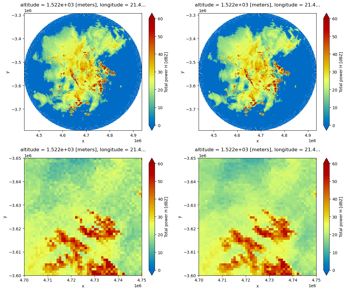

HVPlot¶

hv.extension('bokeh')
hv.output(widget_location="bottom")

swpx = swp_nearest.chunk()
display(swpx)

dbz_opts = dict(
    cmap="HomeyerRainbow", 
    clim=(0, 60), 
    aspect=1
)

vrad_opts = dict(
    cmap="Seismic", 
    clim=(-15, 15), 
    aspect=1
)

wrad_opts = dict(
    cmap="Seismic", 
    clim=(0, 15), 
    aspect=1
)

zdr_opts = dict(
    cmap="HomeyerRainbow", 
    clim=(-0.5, 5), 
    aspect=1
)

rho_opts = dict(
    cmap="plasmidis", 
    clim=(0.0, 1.0), 
    aspect=1
)

phi_opts = dict(
    cmap="Seismic", 
    clim=(0, 60), 
    aspect=1
)

kdp_opts = dict(
    cmap="Seismic", 
    clim=(-0.5, 2), 
    aspect=1
)

moment = swp_nearest["DBTH"].hvplot(x="x", y="y", 
                                   widget_type="scrubber", 
                                   rasterize=True,
                                   widget_location='bottom',
                                   frame_width=500,
                                   **dbz_opts,
                                  )

moment

Write Gridded Data¶

Finally, we write out the data to disk (NetCDF4) for later compositing.

outname_nearest = f"{prefix}_nearest.nc"
swp_nearest.to_netcdf(outname_nearest)

outname_idw = f"{prefix}_idw.nc"
swp_idw.to_netcdf(outname_idw)

swp1 = xr.open_dataset(outname_nearest)
display(swp1)

swp2 = xr.open_dataset(outname_idw)
display(swp2)

Stratiform Case 2014

Stratiform Case 2014¶

Claim Data¶

Georeference¶

Quality Assurance and Quality Control¶

Radar Corrections¶

Quantitative Precipitation Estimation (QPE)¶

Gridding¶

Create cartesian dataset¶

Get KDTree mapping¶

Run Interpolator¶

Plot Gridded Data¶

Matplotlib¶

HVPlot¶

Write Gridded Data¶

Composite¶