Composite To Grid — with QC¶

Same as Composite To Grid, but the reflectivity is quality-controlled and converted to rain rate in radar coordinates before it is gridded and composited. The chain is

open polar  →  QC (attenuation)  →  QPE (Z-R)  →  grid  →  composite

The compositing itself is unchanged — the two radars are still stacked along a radar dimension and reduced with max.

import warnings

import cmweather
import icechunk
import numpy as np
import pyproj
import rioxarray  # noqa: F401 -- registers the .rio accessor used by write_crs
import xarray as xr
import xradar as xd
import matplotlib.pyplot as plt
import hvplot.xarray  # noqa: F401 - registers the .hvplot accessor
import holoviews as hv

import wradlib as wrl

hv.extension("bokeh")
warnings.filterwarnings("ignore")

Claim Data¶

We use the ARCO data from Data Access — Serbian Rainbow Radar directly, in polar (radar) coordinates, because the QC below has to be applied before gridding.

OSN_ENDPOINT = "https://umn1.osn.mghpcc.org"
BUCKET = "nexrad-arco"

# prefix = "Fgora"  # single-pol, 12 sweeps × 360 az × 250 range, 2014 + 2017 + 2026
# prefix = "jastrebac_250m"  # dual-pol, 12 × 360 × 1000, 2014 only
prefix = "jastrebac_500m"  # dual-pol, 12 × 360 × 500,  2017 + 2026

Get Lowest Sweep¶

sweep = "sweep_0"

Get Case¶

case = "2017"
ipol = "nearest"

The two radars are read into a DataTree, one node each, exactly as before — only now the nodes hold polar sweeps rather than pre-gridded fields.

prefixes = {"jastrebac": prefix, "fgora": "Fgora"}

x0 = 3760756.2464729655
y0 = -2656141.3006878751

proj_laea = pyproj.CRS.from_proj4(
    "+proj=laea +lat_0=52 +lon_0=10 "
    f"+x_0={x0} "
    f"+y_0={y0} "
    "+a=6378137 +b=6356752.3141403701 +units=m +no_defs"
)
proj_laea = wrl.georef.ensure_crs(proj_laea)


def open_polar(store):
    """Open one radar's sweep for the selected case, georeferenced onto the LAEA grid."""
    storage = icechunk.s3_storage(
        bucket=BUCKET,
        prefix=store,
        endpoint_url=OSN_ENDPOINT,
        region="us-east-1",
        anonymous=True,
        force_path_style=True,
    )
    repo = icechunk.Repository.open(storage)
    dtree = xr.open_datatree(
        repo.readonly_session("main").store,
        engine="zarr",
        consolidated=False,
        chunks={},
    )
    root = next(iter(dtree.keys())).split("/")[0]
    ds = dtree[f"{root}/{sweep}"].to_dataset(inherit="all_coords").sel(vcp_time=case)
    # DBZH drives the QPE; uPhiDP/RHOHV are read only where they exist (Jastrebac), to
    # let the attenuation correction use the phase-constrained ZPHI method.
    moments = ["DBZH"] + [m for m in ("uPhiDP", "RHOHV") if m in ds]
    swp = ds[moments].load().wrl.georef.georeference(crs=proj_laea)
    swp = swp.rename(crs_wkt="spatial_ref")
    swp.z.attrs = xd.model.get_altitude_attrs()
    return swp.sortby("vcp_time")


ptree = xr.DataTree()
for radar, store in prefixes.items():
    ptree[radar] = open_polar(store)
    print(f"{radar:10} {store:16} {dict(ptree[radar].ds.sizes)}")

jastrebac  jastrebac_500m   {'vcp_time': 35, 'azimuth': 360, 'range': 500}

fgora      Fgora            {'vcp_time': 38, 'azimuth': 360, 'range': 250}

ptree

Quality Control¶

Attenuation correction in radar coordinates, using the modified Krämer scheme from Attenuation correction - Single Pol: constrained in both corrected reflectivity (≤ 59 dBZ) and path-integrated attenuation (≤ 10 dB).

Where $\Phi_{DP}$ is available (Jastrebac) we use the ZPHI method from Attenuation correction - Dual Pol. $\Phi_{DP}$ is a path-integrated quantity that is itself unaffected by attenuation, so it constrains the correction and it cannot run away — unlike the gate-by-gate forward integration, which on this data diverges to infinite PIA.

Fruška Gora is single-polarisation and has no $\Phi_{DP}$ , so it falls back to the constrained scheme of Attenuation correction - Single Pol.

dbz_cap = 59.0
alpha = 0.02   # dB/deg, S band -- as in attenuation_dual_pol.md
b_zphi = 0.62


def attenuation_zphi(swp):
    """Phase-constrained ZPHI attenuation (dual-pol). Bounded by construction."""
    mask = swp.RHOHV >= 0.7
    phimask = swp.uPhiDP.where(mask)
    dbzmask = swp.DBZH.where(mask)
    ah = wrl.atten.specific_attenuation_zphi(
        phimask, dbzmask, alpha=alpha, b=b_zphi, rng=5000.0
    )
    dr = np.diff(ah.range)[0] / 1000.0
    return 2 * (ah.fillna(0) * dr).cumsum(dim="range")


def attenuation_constrained(swp):
    """Single-pol fallback -- see the warning above for the two guards.

    The k-Z coefficients are the values from attenuation_single_pol.md divided by ten.
    Those are C/X-band scale (wradlib's own default a_max is 1.67e-4, for X band) and
    over-correct these S-band radars by an order of magnitude. Calibrating against ZPHI
    on Jastrebac -- same make and band, but with the phase constraint available -- gives:

        a_max      mean PIA     vs ZPHI
        5.0e-5      1.366 dB     11.00x
        1.0e-5      0.293 dB      2.36x
        5.0e-6      0.146 dB      1.17x   <- matches across the distribution
        2.0e-6      0.060 dB      0.49x

    ZPHI reference over the same scans: mean 0.124 dB, p99 1.20, max 2.89.
    """
    gate_length = np.diff(swp.range)[0] / 1000.0
    dbz = swp.DBZH.fillna(-32.0)          # -32 dBZ is the archive's no-echo floor
    pia = xr.concat(
        [
            dbz.isel(vcp_time=slice(i, i + 1)).wrl.atten.correct_attenuation_constrained(
                a_max=5.0e-6,
                a_min=2.0e-6,
                n_a=100,
                b_max=0.75,
                b_min=0.65,
                n_b=6,
                gate_length=gate_length,
                constraints=[wrl.atten.constraint_dbz, wrl.atten.constraint_pia],
                constraint_args=[[dbz_cap], [10.0]],
            )
            for i in range(swp.sizes["vcp_time"])
        ],
        dim="vcp_time",
    )
    return pia


for radar in ptree.children:
    swp = ptree[radar].to_dataset(inherit="all_coords")
    if "uPhiDP" in swp and "RHOHV" in swp:
        pia, method = attenuation_zphi(swp), "ZPHI"
    else:
        pia, method = attenuation_constrained(swp), "constrained"
    pia = pia.where(np.isfinite(swp.DBZH))   # keep unmeasured gates masked
    ptree[radar] = swp.assign(
        PIA=pia,
        DBZH_corr=(swp.DBZH + pia.fillna(0)).clip(max=dbz_cap),
    )
    finite = np.isfinite(pia.values)
    print(f"{radar:10} {method:12} PIA max {np.nanmax(pia.values[finite]):6.2f} dB  "
          f"mean {np.nanmean(pia.values[finite]):6.3f} dB  "
          f"non-finite {100 * (~finite).mean():.2f}%")

jastrebac  ZPHI         PIA max   4.42 dB  mean  0.171 dB  non-finite 0.06%

fgora      constrained  PIA max   5.52 dB  mean  0.275 dB  non-finite 2.63%

vcp = 0
fig, axs = plt.subplots(2, 3, figsize=(16, 9))
kwargs = dict(vmin=0, vmax=60, cmap="HomeyerRainbow")
for row, radar in enumerate(ptree.children):
    ds = ptree[radar].ds
    ds.DBZH.isel(vcp_time=vcp).wrl.vis.plot(ax=axs[row, 0], **kwargs)
    axs[row, 0].set_title(f"{radar} - DBZH")
    ds.DBZH_corr.isel(vcp_time=vcp).wrl.vis.plot(ax=axs[row, 1], **kwargs)
    axs[row, 1].set_title(f"{radar} - attenuation corrected")
    ds.PIA.isel(vcp_time=vcp).wrl.vis.plot(ax=axs[row, 2], vmin=0, vmax=5, cmap="viridis")
    axs[row, 2].set_title(f"{radar} - PIA (dB)")
    for ax in axs[row]:
        ax.set_aspect("equal")
fig.tight_layout()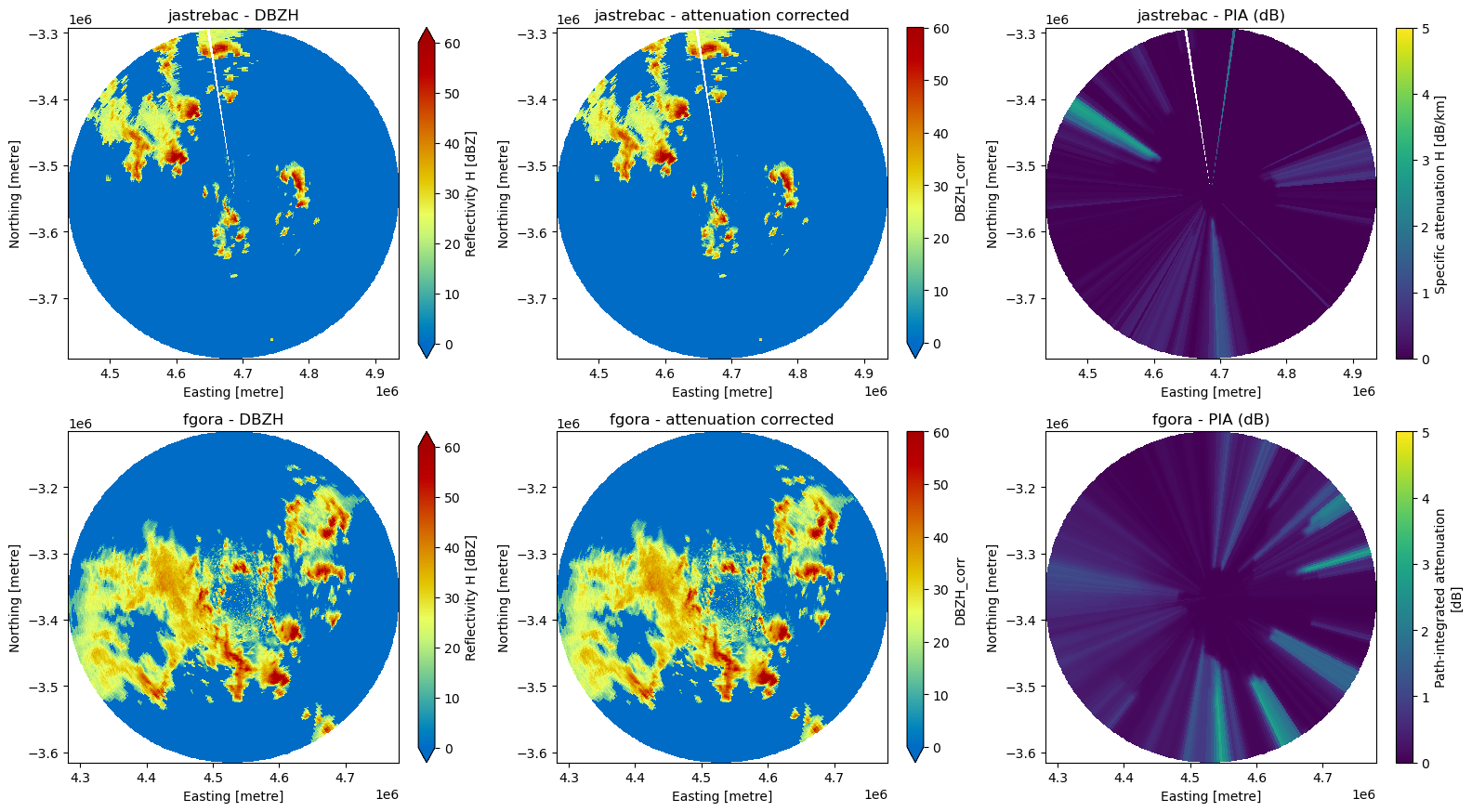

QPE¶

Marshall & Palmer Marshall & Palmer (1948) $Z = a R^b$ with $a=200$ , $b=1.6$ , still in radar coordinates — see Quantitative Precipitation Estimation (QPE).

for radar in ptree.children:
    ds = ptree[radar].to_dataset(inherit="all_coords")
    rain_rate = ds.DBZH_corr.wrl.trafo.idecibel().wrl.zr.z_to_r(a=200.0, b=1.6)
    rain_rate.attrs.update(units="mm/h", long_name="Rain rate (Marshall-Palmer)")
    ptree[radar] = ds.assign(rain_rate=rain_rate)
    v = rain_rate.values[np.isfinite(rain_rate.values)]
    print(f"{radar:10} R median {np.median(v):6.3f}  p99 {np.percentile(v, 99):7.2f}  "
          f"max {v.max():7.2f} mm/h")

jastrebac  R median  0.000  p99   35.40  max  177.56 mm/h
fgora      R median  0.268  p99   31.30  max  177.56 mm/h

Gridding¶

Now the QC’d rain rate goes onto the common cartesian grid, following Gridding Polar Data. Both radars are cut from the same lattice, so their grids share exact coordinates.

nx = 6500
ny = 5300
res = 1000.0

x = x0 + (np.arange(nx) - nx / 2 + 0.5) * res
y = y0 + (np.arange(ny) - ny / 2 + 0.5) * (-res)

ctree = xr.DataTree()
for radar in ptree.children:
    swp = ptree[radar].to_dataset(inherit="all_coords")
    cart = xr.Dataset(coords={"x": ("x", x), "y": ("y", y)}).chunk(x=500, y=500)
    cart = cart.rio.write_crs(proj_laea)
    cart = cart.sel(
        x=slice(swp.x.min(), swp.x.max()),
        y=slice(swp.y.max(), swp.y.min()),
    )
    src = swp[["rain_rate", "DBZH_corr"]]   # both fields ride the same KDTree mapping
    mapping = src.wrl.ipol.get_mapping(cart, k=4)
    ds = src.wrl.ipol.interpolate(mapping, method=ipol).compute()
    ds = ds.assign_coords(vcp_time=ds.vcp_time.dt.floor("5min")).sortby("vcp_time")
    ctree[radar] = ds
    print(f"{radar:10} -> {dict(ds.sizes)}")

jastrebac  -> {'vcp_time': 35, 'y': 499, 'x': 499}

fgora      -> {'vcp_time': 38, 'y': 499, 'x': 499}

ctree

Plot Overview¶

fig, axs = plt.subplots(1, 2, figsize=(12, 5), sharey=True)
ax = axs.flat[1]
ctree["jastrebac"].ds.rain_rate[0].wrl.vis.plot(ax=ax, vmin=0, vmax=30)
ax.set_title("Radar Jastrebac")
ax.set_xlim(min(ctree["fgora"].ds.x.min(), ctree["jastrebac"].ds.x.min()), max(ctree["fgora"].ds.x.max(), ctree["jastrebac"].ds.x.max()))
ax.set_ylim(min(ctree["fgora"].ds.y.min(), ctree["jastrebac"].ds.y.min()), max(ctree["fgora"].ds.y.max(), ctree["jastrebac"].ds.y.max()))
ax = axs.flat[0]
ctree["fgora"].ds.rain_rate[0].wrl.vis.plot(ax=ax, vmin=0, vmax=30)
ax.set_title("Radar Fruŝka Gora")
ax.set_xlim(min(ctree["fgora"].ds.x.min(), ctree["jastrebac"].ds.x.min()), max(ctree["fgora"].ds.x.max(), ctree["jastrebac"].ds.x.max()))
ax.set_ylim(min(ctree["fgora"].ds.y.min(), ctree["jastrebac"].ds.y.min()), max(ctree["fgora"].ds.y.max(), ctree["jastrebac"].ds.y.max()))

(-3790641.300687875, -3116641.300687875)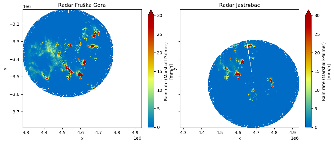

Compositing¶

Before compositing we combine the two radar grids into one Dataset.

radars = xr.DataArray(ctree.children, dims="radar")
radargrids = xr.concat([ctree[radar].ds.rain_rate for radar in ctree.children], dim=radars)
dbzgrids = xr.concat([ctree[radar].ds.DBZH_corr for radar in ctree.children], dim=radars)

radargrids

Then we finally reduce over the radar dimension to create the final output. Both fields are reduced the same way, and because $Z \rightarrow R$ is monotonic, max picks the same radar for each cell in both — the two composites stay mutually consistent.

composite = radargrids.max("radar")
dbz_composite = dbzgrids.max("radar")
n_radars = radargrids.notnull().sum("radar").astype("uint8")

composite

Plot Result¶

Always check your source data! In our case the first timestep is only available for Fruška_Gora Radar, Jastrebac Radar is missing.

composite.isel(vcp_time=3).hvplot.quadmesh(
    x="x",
    y="y",
    rasterize=True,
    cmap="ChaseSpectral",
    clim=(0, 100),
    frame_width=550,
    frame_height=500,
    aspect="equal",

)

In the second timestep, Jastrebac is contained in the composite.

Write Composite¶

Both composites go into a single, self-describing Zarr store following CF conventions: standard names and units on every variable, a lambert_azimuthal_equal_area grid mapping so the projection travels with the data, and provenance in the global attributes. Anyone opening it can georeference and interpret it without needing this notebook.

comp = xr.Dataset(
    {
        "DBZH": dbz_composite.astype("float32"),
        "rain_rate": composite.astype("float32"),
        "n_radars": n_radars,
    }
)

comp["DBZH"].attrs = {
    "standard_name": "equivalent_reflectivity_factor",
    "long_name": "Attenuation-corrected horizontal reflectivity composite",
    "units": "dBZ",
    "grid_mapping": "spatial_ref",
    "cell_methods": "radar: maximum",
}
comp["rain_rate"].attrs = {
    "standard_name": "rainfall_rate",
    "long_name": "Rain rate composite from Marshall-Palmer Z-R",
    # CF's canonical units for rainfall_rate are kg m-2 s-1; mm h-1 is the conventional
    # radar-QPE form and assumes a water density of 1000 kg m-3 (1 mm h-1 = 2.778e-4).
    "units": "mm h-1",
    "grid_mapping": "spatial_ref",
    "cell_methods": "radar: maximum",
    "zr_a": 200.0,
    "zr_b": 1.6,
}
comp["n_radars"].attrs = {
    "long_name": "Number of radars contributing to each cell",
    "units": "1",
    "grid_mapping": "spatial_ref",
    "comment": "0 = no data, 1 = single radar, 2 = both radars in the overlap",
}
comp["x"].attrs = {
    "standard_name": "projection_x_coordinate",
    "long_name": "Easting",
    "units": "m",
    "axis": "X",
}
comp["y"].attrs = {
    "standard_name": "projection_y_coordinate",
    "long_name": "Northing",
    "units": "m",
    "axis": "Y",
}
comp["vcp_time"].attrs = {"standard_name": "time", "long_name": "Volume time", "axis": "T"}

# rioxarray writes the CF grid mapping variable (grid_mapping_name, crs_wkt, datum
# parameters) so the projection is carried inside the store.
comp = comp.rio.write_crs(proj_laea, grid_mapping_name="spatial_ref")

comp.attrs = {
    "Conventions": "CF-1.10",
    "title": f"ERAD2026 gridded radar composite ({case}) - reflectivity and rain rate",
    "institution": "Open Radar Science Short Course, ERAD2026",
    "source": (
        f"Fruska Gora + Jastrebac {sweep} (0.5 deg), Serbian RHMZ; "
        f"ARCO stores s3://{BUCKET}/{{Fgora, {prefix}}}"
    ),
    "history": (
        "attenuation correction (ZPHI where PHIDP available, else constrained k-Z with "
        "S-band coefficients); Marshall-Palmer Z-R (a=200, b=1.6); reflectivity capped at "
        f"{dbz_cap} dBZ before Z-R; nearest-neighbour gridding to 1 km LAEA; "
        "composited as maximum over radars"
    ),
    "references": "https://openradarscience.org/erad2026",
    "comment": (
        "Lowest sweep only. Rain rate is single-polarisation Z-R throughout, so it is best "
        "justified in stratiform rain and least so in convective cores."
    ),
}
display(comp)

outname_composit = "composite.zarr"
comp.to_zarr(outname_composit, mode="w", zarr_format=3, consolidated=False)

The published store stands on its own — the CRS, units and standard names all travel with it. We read it straight from the cloud rather than from disk:

grd = xr.open_zarr(
    f"s3://{BUCKET}/composite.zarr",
    storage_options={"anon": True, "client_kwargs": {"endpoint_url": OSN_ENDPOINT}},
    consolidated=False,
    decode_coords="all",
    chunks={},
)
grd

Next Steps¶

You’ve completed the QC + QPE compositing workflow for the selected dataset. Return to case selection step, change accordingly, and rerun the notebook.

References¶

Marshall, J. S., & Palmer, W. M. K. (1948). THE DISTRIBUTION OF RAINDROPS WITH SIZE. Journal of Meteorology, 5(4), 165–166. https://doi.org/10.1175/1520-0469(1948)005<;0165:tdorws>2.0.co;2