


Quasi-Vertical Profiles (QVP)
Quasi-Vertical Profiles (QVPs) turn the PPI volumes a radar already collects into a time-height view of the atmosphere above it, without needing dedicated RHI scans. The technique was introduced by Ryzhkov et al. Ryzhkov et al. (2016): at a single, sufficiently high and fixed elevation angle, reflectivity and the polarimetric moments are averaged around the full azimuthal sweep into one vertical profile, and stacking these profiles in time reveals how the vertical structure evolves as precipitation passes over the radar.
Prerequisites
| Concepts | Importance | Notes |
|---|---|---|
| Xarray Basics | Necessary | Working with radar DataTrees and azimuthal averaging |
| Polarimetric Radar Variables | Helpful | Interpreting ZDR, KDP, RHOHV |
Time to learn: 15 minutes
Overview
A QVP is the azimuthal mean of a polarimetric moment at a fixed elevation, evolving in time:
Ryzhkov et al. Ryzhkov et al. (2016) used this technique to track the melting layer and dendritic growth zone (roughly -10 to -15 degrees Celsius) as precipitation evolves. In that layer, ice crystals grow into dendrites and begin to aggregate as they fall and partially melt; in a QVP this shows up as a ZDR increase (up to 1.5-2 dB), a RHOHV decrease, and a strong vertical gradient in Z, sometimes accompanied by a nonzero KDP as the vertical phase gradient responds to the changing hydrometeor population. Because a QVP only needs the routine PPI volumes a radar already collects, it lets researchers examine the time evolution of these microphysical processes continuously, and compare polarimetric radar observations directly against vertically pointing remote sensors.
QVPs assume precipitation is approximately uniform in a ring around the radar, so they are most reliable in widespread, layered precipitation. For an isolated convective cell the azimuthal average mixes in-storm and clear-air rays, but the technique remains a useful way to track how a storm’s vertical structure evolves as it approaches, passes over, and recedes from the radar — which is why we apply it here to the Jastrebac dual-polarization convective case (Convective Case 2017) rather than the single-polarization data used for QPE.
Claim Data
We use the ARCO data provided in Data Access — Serbian Rainbow Radar.
OSN_ENDPOINT = "https://umn1.osn.mghpcc.org"
BUCKET = "nexrad-arco"
prefix = "jastrebac_500m" # dual-pol, 12 × 360 × 500, 2017 + 2026 — convective case
storage = icechunk.s3_storage(
bucket=BUCKET,
prefix=prefix,
endpoint_url=OSN_ENDPOINT,
region="us-east-1",
anonymous=True,
force_path_style=True,
)
repo = icechunk.Repository.open(storage)
dtree = xr.open_datatree(
repo.readonly_session("main").store,
engine="zarr",
consolidated=False,
chunks={},
).sel(vcp_time="2017")
display(dtree)
root = next(iter(dtree.keys())).split("/")[0]Select the Highest Elevation
QVPs are computed from the steepest routinely available elevation angle: a steeper beam needs less range to reach a given height, which reduces horizontal drift and keeps the assumption that one azimuthal sweep samples a roughly co-located vertical column.
sweeps = sorted(dtree[root].children, key=lambda s: int(s.split("_")[-1]))
sweep = sweeps[-1]

swp = dtree[f"{root}/{sweep}"].to_dataset(inherit="all_coords")
elevation_deg = float(swp.sweep_fixed_angle.isel(vcp_time=0))
print(f"Using {sweep} at {elevation_deg:.1f}\N{DEGREE SIGN} elevation")
display(swp)
Using sweep_11 at 25.0° elevation
Quality Control
qc_mask = swp.RHOHV >= 0.7
zdr = swp.ZDR.where(qc_mask)
rhohv = swp.RHOHV.where(qc_mask)
kdp = swp.KDP.where(qc_mask & (swp.KDP > -9))
Compute the QVP
Reflectivity must be averaged in linear units and converted back to dB afterwards — averaging directly in dB would bias the mean low, since dB compresses the dynamic range of the underlying (linear) received power. Height above the radar follows from simple trigonometry on the fixed elevation angle and range: .
def azimuthal_mean(da, is_db=False):
    lin = 10 ** (da / 10) if is_db else da
    out = lin.mean("azimuth", skipna=True)
    return 10 * np.log10(out.where(out > 0)) if is_db else out

elevation = np.deg2rad(elevation_deg)
height = (swp.range * np.sin(elevation) / 1000).assign_attrs(units="km", long_name="Height above radar")

qvp = xr.Dataset(
    {
        "DBZH": azimuthal_mean(swp.DBZH, is_db=True),
        "ZDR": azimuthal_mean(zdr),
        "RHOHV": azimuthal_mean(rhohv),
        "KDP": azimuthal_mean(kdp),
    }
).assign_coords(height=height)
qvp = qvp.where(qvp.height <= 15, drop=True)
display(qvp)Visualize the Vertical Structure
fig, axes = plt.subplots(2, 2, figsize=(14, 9), sharex=True, sharey=True)

qvp.DBZH.plot(ax=axes[0, 0], x="vcp_time", y="height", cmap="HomeyerRainbow", vmin=0, vmax=60)
axes[0, 0].set_title("QVP - Reflectivity (DBZH)")

qvp.ZDR.plot(ax=axes[0, 1], x="vcp_time", y="height", cmap="HomeyerRainbow", vmin=0, vmax=8)
axes[0, 1].set_title("QVP - Differential Reflectivity (ZDR)")

qvp.RHOHV.plot(ax=axes[1, 0], x="vcp_time", y="height", cmap="plasmidis", vmin=0.7, vmax=1)
axes[1, 0].set_title("QVP - Correlation Coefficient (RHOHV)")

qvp.KDP.plot(ax=axes[1, 1], x="vcp_time", y="height", cmap="seismic", vmin=-2, vmax=2)
axes[1, 1].set_title("QVP - Specific Differential Phase (KDP)")

for ax in axes[0, :]:
    ax.set_xlabel("")
for ax in axes[1, :]:
    ax.set_xlabel("Time (UTC)")
    ax.tick_params(axis="x", rotation=30)
for ax in axes[:, 0]:
    ax.set_ylabel("Height (km)")
for ax in axes[:, 1]:
    ax.set_ylabel("")
fig.tight_layout()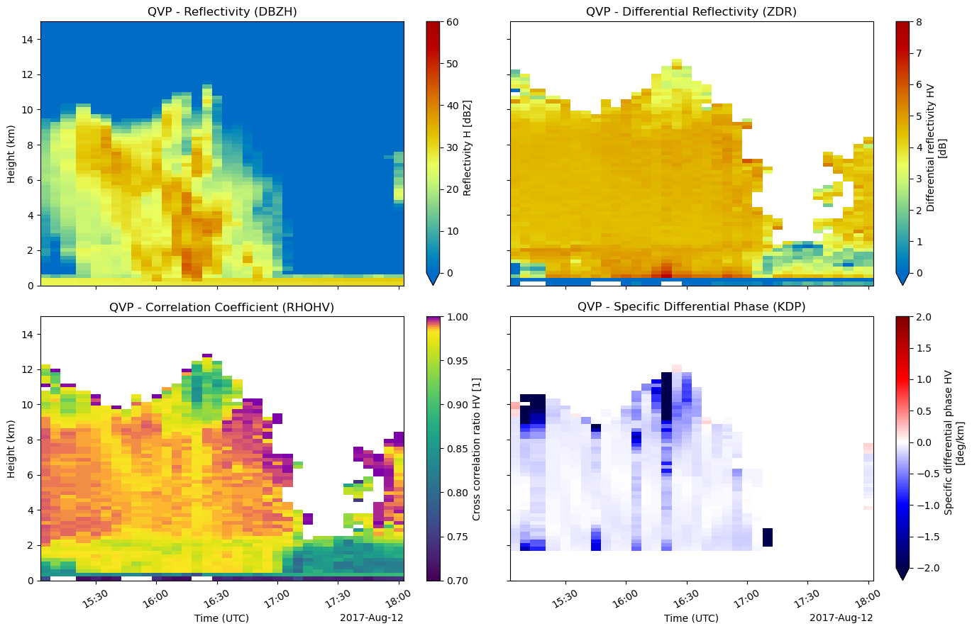
Next Steps
You’ve computed a QVP for the convective case at the highest available elevation. Return to the sweep selection step to try a lower elevation angle — you’ll need a longer range to reach the same height, trading vertical resolution for a wider footprint around the radar.
- Ryzhkov, A., Zhang, P., Reeves, H., Kumjian, M., Tschallener, T., Trömel, S., & Simmer, C. (2016). Quasi-Vertical Profiles—A New Way to Look at Polarimetric Radar Data. Journal of Atmospheric and Oceanic Technology, 33(3), 551–562. 10.1175/jtech-d-15-0020.1