Attenuation correction - Dual Pol¶

Weather radar reflectivity measurements are affected by propagation effects, most importantly attenuation due to hydrometeors along the radar beam. In X-band and C-band radar applications, this can lead to significant underestimation of reflectivity at long range and in heavy precipitation.

import cmweather
import numpy as np
import matplotlib.pyplot as plt
import wradlib as wrl
import xarray as xr
import xradar as xd
import fsspec
import icechunk
import holoviews as hv
import hvplot
import hvplot.xarray
import warnings
warnings.filterwarnings("ignore")

Claim Data and Overview¶

We use the ARCO data provided in Data Access — Serbian Rainbow Radar. Please refer to this notebook for details of access.

OSN_ENDPOINT = "https://umn1.osn.mghpcc.org"
BUCKET = "nexrad-arco"

# prefix = "jastrebac_250m"  # dual-pol, 12 × 360 × 1000, 2014 only
prefix = "jastrebac_500m"  # dual-pol, 12 × 360 × 500,  2017 + 2026

storage = icechunk.s3_storage(
    bucket=BUCKET,
    prefix=prefix,
    endpoint_url=OSN_ENDPOINT,
    region="us-east-1",
    anonymous=True,
    force_path_style=True,
)
repo = icechunk.Repository.open(storage)
dtree = xr.open_datatree(
    repo.readonly_session("main").store,
    engine="zarr",
    consolidated=False,
    chunks={},
)
display(dtree)
root = next(iter(dtree.keys())).split("/")[0]

Get lowest elevation sweep¶

First we get the lowest sweep and do some georeferencing.

swp = (
    dtree[f"{root}/sweep_0"]
    .to_dataset()
    .assign_coords(dtree[root].coords)
    .assign_coords(sweep_mode="azimuth_surveillance")
    .wrl.georef.georeference(crs=wrl.georef.get_earth_projection())
)
swp.x.attrs = xd.model.get_longitude_attrs()
swp.y.attrs = xd.model.get_latitude_attrs()
swp.z.attrs = xd.model.get_altitude_attrs()
display(swp)

mask = swp.RHOHV >= 0.7
phimask = swp.uPhiDP.where(mask)
dbzmask = swp.DBZH.where(mask)

vcp = 10

Overview Plot¶

We can clearly see, that $\Phi_{DP}$ (left) has been corrected for $\Phi^{sys}_{DP}$ .

fig, (ax1, ax2) = plt.subplots(1, 2, figsize=(16, 8))
phimask.isel(vcp_time=vcp).wrl.vis.plot(ax=ax1, vmin=90, vmax=300)
ax1.set_title("Uncorrected Differential Phase")
swp.PHIDP.where(mask).isel(vcp_time=vcp).wrl.vis.plot(ax=ax2, vmin=0, vmax=200)
ax2.set_title("Corrected Differential Phase")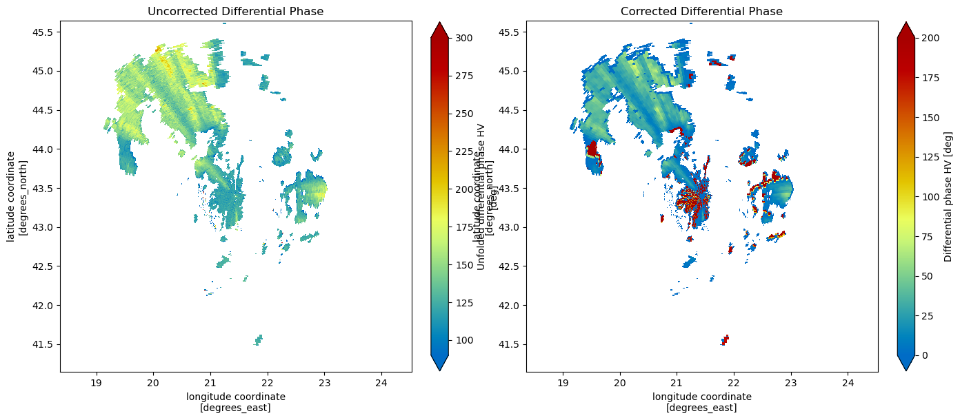

fig, (ax1, ax2) = plt.subplots(1, 2, figsize=(16, 8))
swp.DBTH.where(mask).isel(vcp_time=vcp).wrl.vis.plot(ax=ax1, vmin=0, vmax=60)
ax1.set_title("Uncorrected Reflectivity")
dbzmask.isel(vcp_time=vcp).wrl.vis.plot(ax=ax2, vmin=0, vmax=60)
ax2.set_title("Corrected Reflectivity")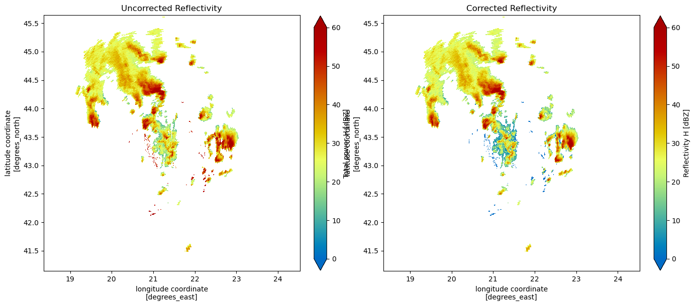

Standard Correction Method¶

Attenuation is most pronounced for X- and C-band weather radars, where phase-based correction methods have become standard (e.g., Jameson (1992); Testud et al. (2000)). Although attenuation at S band is generally much smaller, the same methodology can be applied to mitigate attenuation during heavy precipitation and to ensure consistency in polarimetric radar processing. A simple phase-based correction is given by

Z^{corr}_{H}(r) = Z^{att}_{H}(r) + \alpha\Phi_{DP}(r)

(1)

Z^{corr}_{DR}(r) = Z^{att}_{DR}(r) + \beta\Phi_{DP}(r)

(2)

Table 1:Ranges of variability of α and β in rain at S, C, and X bands

Band	α range (dB deg⁻¹)	⟨α⟩ (dB deg⁻¹)	β range (dB deg⁻¹)	⟨β⟩ (dB deg⁻¹)
S band	0.015–0.04	0.02	0.0025–0.009	0.004
C band	0.05–0.18	0.08	0.008–0.10	0.02
X band	0.14–0.35	0.28	0.03–0.06	0.05

Source: Ryzhkov & Zrnic (2019), Radar Polarimetry for Weather Observations (Springer)

Specific Attenuation via ZPHI method¶

The ZPHI method provides a physically constrained approach to estimate specific attenuation from the joint evolution of reflectivity ( $Z_H$ ) and differential phase shift ( $\Phi_{DP}$ ). It exploits the fact that $\Phi_{DP}$ is a path-integrated quantity that is not directly affected by attenuation and can therefore be used as a robust constraint.

In this notebook, we demonstrate a complete ZPHI processing chain including:

estimation of total differential phase shift ( $\Delta \Phi_{DP}^{tot}$ )
reconstruction of $\Phi_{DP}^{cal}$ from $K_{DP}$ (when needed)
retrieval of specific attenuation ( $A_H$ / $A_V$ )

The workflow follows established formulations from Testud et al. (2000), Ryzhkov et al. (2014), and Diederich et al. (2015).

Total differential phase shift ( $\Delta \Phi_{DP}^{tot}$ )¶

dphi = phimask.wrl.dp.delta_phidp(5000.)
display(dphi)

fig, (ax1, ax2) = plt.subplots(2, 1, figsize=(16, 8))
dphi.first.isel(vcp_time=vcp).plot(label="first", ax=ax1)
dphi.last.isel(vcp_time=vcp).plot(label="last", ax=ax1)
ax1.grid()
ax1.legend()
dphi.dphi.isel(vcp_time=vcp).plot(ls="-", marker=".", label="delta", ax=ax2)
ax2.grid()
ax2.legend()
plt.tight_layout()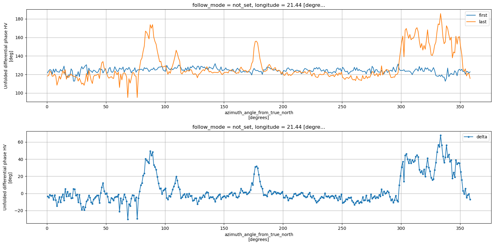

Overview in Polar Domain¶

fig = plt.figure(figsize=(20, 14))
ax1 = plt.subplot(231, projection="polar")
ax2 = plt.subplot(232, projection="polar")
ax3 = plt.subplot(233, projection="polar")
# set the lable go clockwise and start from the top
ax1.set_theta_zero_location("N")
ax2.set_theta_zero_location("N")
ax3.set_theta_zero_location("N")
# clockwise
ax1.set_theta_direction(-1)
ax2.set_theta_direction(-1)
ax3.set_theta_direction(-1)

theta = np.linspace(0, 2 * np.pi, num=360, endpoint=False)
ax1.plot(theta, dphi.first_idx.isel(vcp_time=vcp), color="b", linewidth=3)
_ = ax1.set_title(r"$\Delta \Phi_{DP}$ - First Index")
ax2.plot(theta, dphi.last_idx.isel(vcp_time=vcp), color="r", linewidth=3)
_ = ax2.set_title(r"$\Delta \Phi_{DP}$ - Last Index")
ax3.plot(theta, dphi.dphi.isel(vcp_time=vcp), color="g", linewidth=3)
_ = ax3.set_title(r"$\Delta \Phi_{DP}^{tot}$")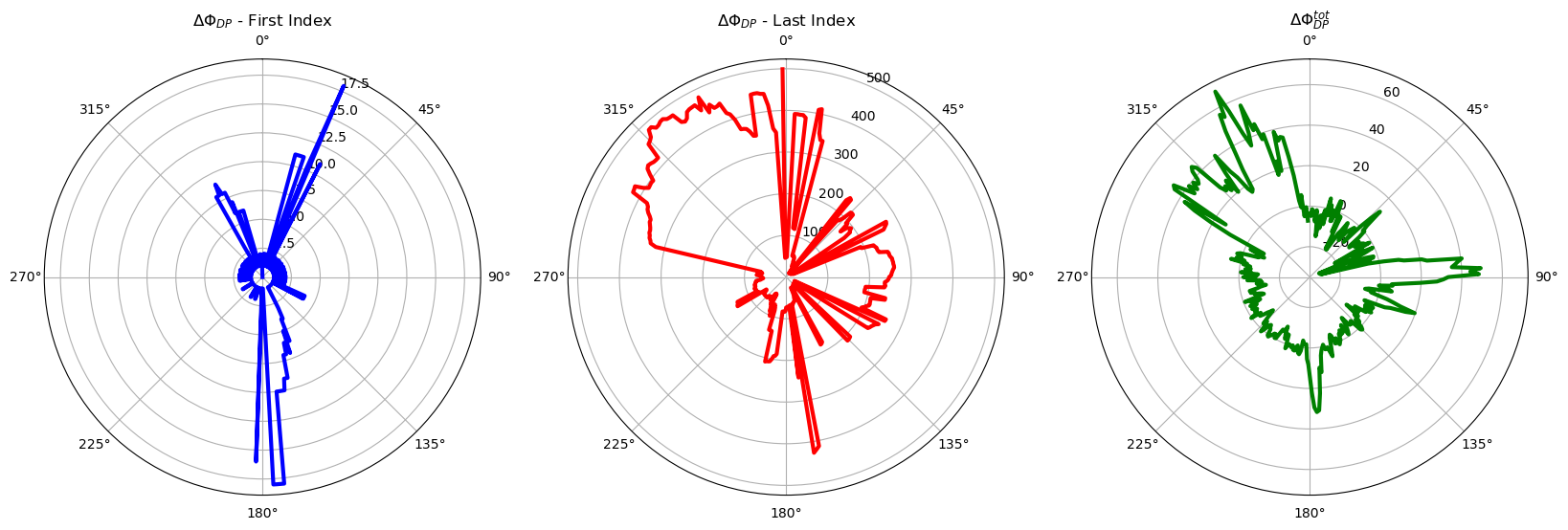

Overview of first and last segments¶

fig, (ax1, ax2) = plt.subplots(2, 1, figsize=(10, 10), sharex=True)
dphi.start_range.isel(vcp_time=vcp).plot(ax=ax1, lw=0.8, c="k")
(dphi.start_range.isel(vcp_time=vcp) + dphi.center_span).plot(ax=ax1, lw=0.8, c="r", ls=":")
dphi.stop_range.isel(vcp_time=vcp).plot(ax=ax1, lw=0.8, c="k")
(dphi.stop_range.isel(vcp_time=vcp) - dphi.center_span).plot(ax=ax1, lw=0.8, c="r", ls=":")
phimask.isel(vcp_time=vcp).plot(ax=ax1, x="azimuth", y="range", cmap="turbo", vmin=90, vmax=300)
ax1.set_title(r"$\Phi_{DP}$ - start/stop")

phimask2 = phimask.where(((phimask.range >= dphi.start_range.isel(vcp_time=vcp)) & (phimask.range <= dphi.start_range.isel(vcp_time=vcp) + dphi.center_span)) |
                         ((phimask.range >= dphi.stop_range.isel(vcp_time=vcp) - dphi.center_span) & (phimask.range <= dphi.stop_range.isel(vcp_time=vcp))))
phimask2.isel(vcp_time=vcp).plot(ax=ax2, x="azimuth", y="range", cmap="turbo", vmin=90, vmax=300)
dphi.start_range.isel(vcp_time=vcp).plot(ax=ax2, lw=0.8, c="k", ls=":")
(dphi.start_range.isel(vcp_time=vcp) + dphi.center_span).plot(ax=ax2, lw=0.8, c="k", ls=":")
dphi.stop_range.isel(vcp_time=vcp).plot(ax=ax2, lw=0.8, c="k", ls=":")
(dphi.stop_range.isel(vcp_time=vcp) - dphi.center_span).plot(ax=ax2, lw=0.8, c="k", ls=":")
ax2.set_title(r"$\Phi_{DP}$ - start/stop - masked")
fig.tight_layout()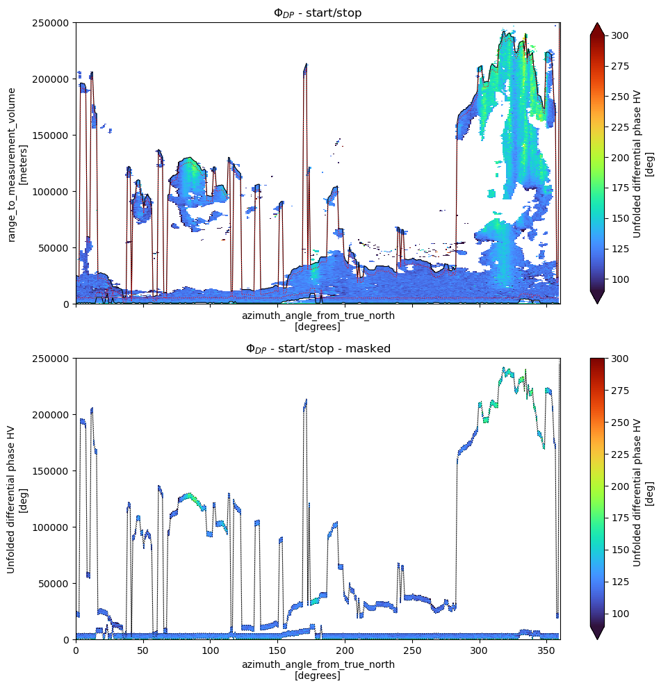

Calculate specific attenuation AH¶

alpha = 0.02
ah = wrl.atten.specific_attenuation_zphi(phimask, dbzmask, alpha=alpha, b=0.62, rng=5000.)

Plot specific attenuation AH¶

ah.isel(vcp_time=vcp).wrl.vis.plot()
plt.gca().set_title(r"$A_{H}$")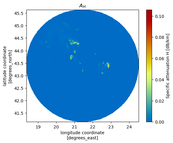

Derive $K_{DP}$ ¶

kdp_ah = ah.fillna(0) / alpha
kdp_ah.attrs = swp.KDP.attrs

kdp_ah.isel(vcp_time=vcp).wrl.vis.plot()
plt.gca().set_title(r"$K_{DP}$")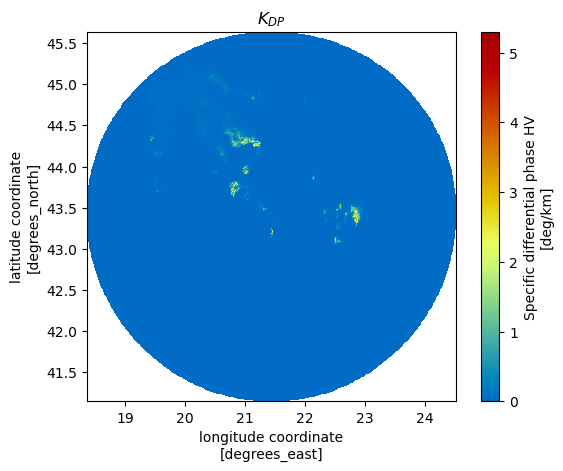

Recalculate $\Phi_{DP}^{cal}$ ¶

phical = kdp_ah.wrl.dp.phidp_from_kdp()
phical = phical.rename("PHIDP_AH")
phical.attrs = swp.PHIDP.attrs

Plot $\Phi_{DP}^{cal}$ ¶

phical.isel(vcp_time=vcp).wrl.vis.plot()
plt.gca().set_title(r"$Phi_{DP}^{cal}$")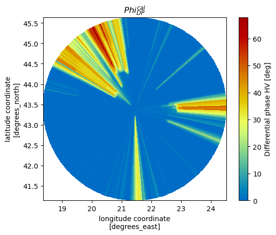

Plot PIA¶

dr = np.diff(ah.range)[0] / 1000
pia_zphi = 2 * (ah.fillna(0) * dr).cumsum(dim="range")
pia_zphi.attrs = wrl.atten._get_path_integrated_attenuation_attrs()
pia_zphi.isel(vcp_time=vcp).wrl.vis.plot()
plt.gca().set_title(r"$PIA$")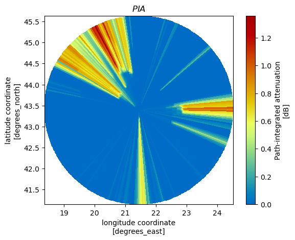

Comparison¶

dbz_kwargs = dict(vmin=0, vmax=60, levels=np.arange(0, 65, 5)) 
fig = plt.figure(figsize=(12, 6))
dbzmask.isel(vcp_time=vcp).wrl.vis.plot(ax=121, **dbz_kwargs)
plt.gca().set_title("DBZH")
dbz_corr = dbzmask + pia_zphi
dbz_corr.attrs = swp.DBZH.attrs
dbz_corr.isel(vcp_time=vcp).wrl.vis.plot(ax=122, **dbz_kwargs)
plt.gca().set_title("DBZH + PIA")
fig.suptitle("ZPHI", fontsize=16)
fig.tight_layout()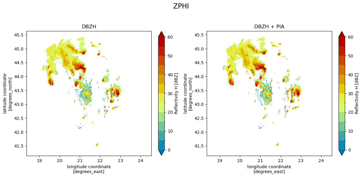

Next Steps¶

You’ve completed the dual pol attenuation correction workflow for the selected dataset. Return to Claim Data and Overview, select the other case study day, and rerun the notebook.

References¶

Jameson, A. R. (1992). The Effect of Temperature on Attenuation-Correction Schemes in Rain Using Polarization Propagation Differential Phase Shift. Journal of Applied Meteorology, 31(9), 1106–1118. https://doi.org/10.1175/1520-0450(1992)031<;1106:teotoa>2.0.co;2
Testud, J., Le Bouar, E., Obligis, E., & Ali-Mehenni, M. (2000). The Rain Profiling Algorithm Applied to Polarimetric Weather Radar. Journal of Atmospheric and Oceanic Technology, 17(3), 332–356. https://doi.org/10.1175/1520-0426(2000)017<;0332:trpaat>2.0.co;2
Ryzhkov, A. V., & Zrnic, D. S. (2019). Radar Polarimetry for Weather Observations. In Springer Atmospheric Sciences. Springer International Publishing. 10.1007/978-3-030-05093-1
Testud, J., Le Bouar, E., Obligis, E., & Ali-Mehenni, M. (2000). The Rain Profiling Algorithm Applied to Polarimetric Weather Radar. Journal of Atmospheric and Oceanic Technology, 17(3), 332–356. https://doi.org/10.1175/1520-0426(2000)017<;0332:trpaat>2.0.co;2
Ryzhkov, A., Diederich, M., Zhang, P., & Simmer, C. (2014). Potential Utilization of Specific Attenuation for Rainfall Estimation, Mitigation of Partial Beam Blockage, and Radar Networking. Journal of Atmospheric and Oceanic Technology, 31(3), 599–619. 10.1175/jtech-d-13-00038.1
Diederich, M., Ryzhkov, A., Simmer, C., Zhang, P., & Trömel, S. (2015). Use of Specific Attenuation for Rainfall Measurement at X-Band Radar Wavelengths. Part I: Radar Calibration and Partial Beam Blockage Estimation. Journal of Hydrometeorology, 16(2), 487–502. 10.1175/jhm-d-14-0066.1

Attenuation correction - Dual Pol

Attenuation correction - Dual Pol¶

Claim Data and Overview¶

Get lowest elevation sweep¶

Overview Plot¶

Standard Correction Method¶

Specific Attenuation via ZPHI method¶

Total differential phase shift (ΔΦDPtot\Delta \Phi_{DP}^{tot}ΔΦDPtot​)¶

Overview in Polar Domain¶

Overview of first and last segments¶

Calculate specific attenuation AH¶

Plot specific attenuation AH¶

Derive KDPK_{DP}KDP​¶

Recalculate ΦDPcal\Phi_{DP}^{cal}ΦDPcal​¶

Plot ΦDPcal\Phi_{DP}^{cal}ΦDPcal​¶

Plot PIA¶

Comparison¶

Next Steps¶

Total differential phase shift ( $\Delta \Phi_{DP}^{tot}$ )¶

Derive $K_{DP}$ ¶

Recalculate $\Phi_{DP}^{cal}$ ¶

Plot $\Phi_{DP}^{cal}$ ¶