Attenuation correction - Single Pol¶

In this notebook, we will compare different approaches to constrain the gate-by-gate retrieval of path-integrated attenuation.

Introduction¶

Rainfall-induced attenuation is a major source of underestimation for radar-based precipitation estimation at C-band and X-band. Unconstrained forward gate-by-gate correction is known to be inherently unstable and thus not suited for unsupervised quality control procedures. Ideally, reference measurements (e.g. from microwave links) should be used to constrain gate-by-gate procedures. However, such attenuation references are usually not available. $\omega radlib$ provides a pragmatic approach to constrain gate-by-gate correction procedures, inspired by the work of Krämer & Verworn (2009). It turned out that these procedures can effectively reduce the error introduced by attenuation, and, at the same time, minimize instability issues Jacobi & Heistermann (2016).

import cmweather
import numpy as np
import matplotlib.pyplot as plt
import wradlib as wrl
import xarray as xr
import xradar as xd
import fsspec
import icechunk
import holoviews as hv
import hvplot
import hvplot.xarray
import warnings
warnings.filterwarnings("ignore")

Claim Data¶

We use the ARCO data provided in Data Access — Serbian Rainbow Radar. Please refer to this notebook for details of access.

OSN_ENDPOINT = "https://umn1.osn.mghpcc.org"
BUCKET = "nexrad-arco"

prefix = "Fgora"  # single-pol, 12 sweeps × 360 az × 250 range, 2014 + 2017 + 2026

storage = icechunk.s3_storage(
    bucket=BUCKET,
    prefix=prefix,
    endpoint_url=OSN_ENDPOINT,
    region="us-east-1",
    anonymous=True,
    force_path_style=True,
)
repo = icechunk.Repository.open(storage)
dtree = xr.open_datatree(
    repo.readonly_session("main").store,
    engine="zarr",
    consolidated=False,
    chunks={},
)
display(dtree)
root = next(iter(dtree.keys())).split("/")[0]

Get lowest elevation sweep¶

First we get the lowest sweep and do some georeferencing.

swp = (
    dtree[f"{root}/sweep_0"]
    .to_dataset()
    .assign_coords(dtree[root].coords)
    .assign_coords(sweep_mode="azimuth_surveillance")
    .wrl.georef.georeference(crs=wrl.georef.get_earth_projection())
).sel(vcp_time="2017")
swp.x.attrs = xd.model.get_longitude_attrs()
swp.y.attrs = xd.model.get_latitude_attrs()
swp.z.attrs = xd.model.get_altitude_attrs()
display(swp)

vcp = 0
gate_length = np.diff(swp.range)[0] / 1000.

azi_slice = (300, 303)
dbz_kwargs = dict(vmin=0, vmax=60, levels=np.arange(0, 65, 5)) 
pia_kwargs = dict(vmin=0, vmax=40, levels=np.arange(0, 45, 5))

dbz = swp.DBZH.isel(vcp_time=vcp)
# plot raw reflectivity
pm = dbz.wrl.vis.plot(**dbz_kwargs)
print(azi_slice[0])
sel = dbz.sel(azimuth=azi_slice[0], method="nearest")
plt.gca().plot(
    [sel.x[0], sel.x[-1]], [sel.y[0], sel.y[-1]], "r-", lw=2
)
plt.title("Raw Reflectivity (dBZ)")
plt.tight_layout()

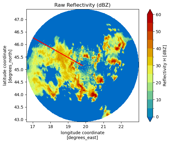
We see a set of convective cells with high rainfall intensity. Let us examine the reflectivity profile along three beams at azimuths 275-277 degree (as marked by the red line in the PPI above).

fig, ax = plt.subplots(1, 1, figsize=(10, 3))
sel = dbz.sel(azimuth=slice(*azi_slice))
sel.plot.line(ax=ax, hue="azimuth")
ax.grid(True, which='both', linestyle='--', alpha=0.7)
ax.set_xlim(float(sel.range.min()), float(sel.range.max()))
ax.set_title("Raw Reflectivity along beams (dBZ)")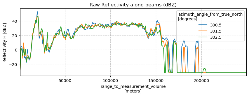

1. Hitschfeld and Bordan¶

Unconstrained gate-by-gate retrieval (1954)

First, we examine the behaviour of the “classical” unconstrained forward correction which is typically referred to Hitschfeld & Bordan (1954), although Hitschfeld and Bordan themselves rejected this approach. The Path Integrated Attenuation (PIA) according to this approach can be obtained as follows:

pia_hibo = dbz.wrl.atten.correct_attenuation_hb(
    coefficients=dict(a=8.0e-5, b=0.731, gate_length=gate_length), mode="warn", thrs=59.0
)

In the coefficients dictionary, we can pass the power law parameters of the A(Z) relation as well as the gate length (in km). If we pass "warn" as the mode argument, we will obtain a warning log in case the corrected reflectivity exceeds the value of argument thrs (dBZ).

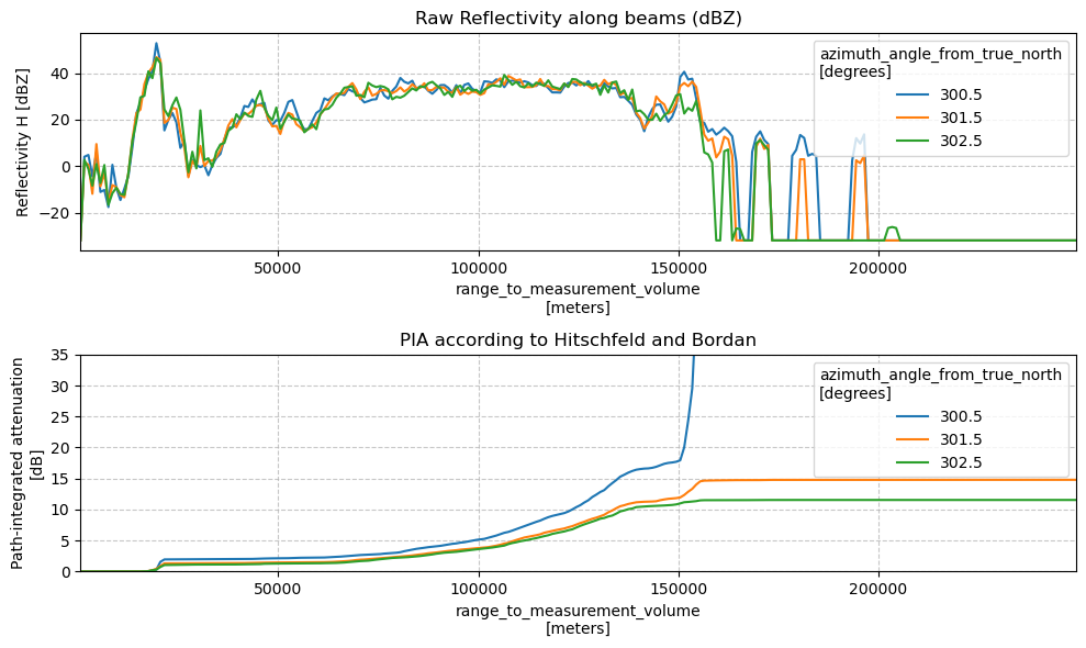
Plotting the result below the reflectivity profile, we obtain the following figure:

fig, (ax1, ax2) = plt.subplots(2, 1, figsize=(10, 6))
sel = dbz.sel(azimuth=slice(*azi_slice))
sel.plot.line(ax=ax1, hue="azimuth")
ax1.grid(True, which='both', linestyle='--', alpha=0.7)
ax1.set_xlim(float(sel.range.min()), float(sel.range.max()))
ax1.set_title("Raw Reflectivity along beams (dBZ)")
sel2 = pia_hibo.sel(azimuth=slice(*azi_slice))
sel2.plot.line(ax=ax2, hue="azimuth")
ax2.grid(True, which='both', linestyle='--', alpha=0.7)
ax2.set_xlim(float(sel.range.min()), float(sel.range.max()))
ax2.set_ylim(0, 35)
ax2.set_title("PIA according to Hitschfeld and Bordan")
plt.tight_layout()

corrected signal over threshold (59.0)

pia_hibo.wrl.vis.plot(**pia_kwargs)
plt.gca().set_title("PIA Hitschfeld & Bordan")

corrected signal over threshold (59.0)

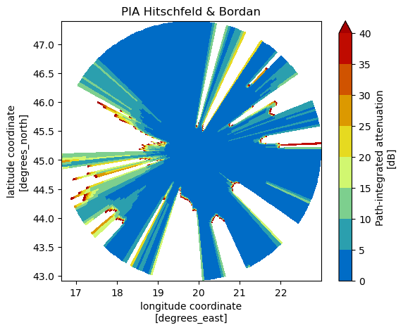
Apparently, slight differences in the reflectivity profile can cause a dramatic change in the behaviour. While at 301.5 and 302.5 degrees azimuth, the retrieval of PIA appears to be fairly stable, the profile of PIA for 300.5 degree demonstrates a case of instability.

2. Harrison¶

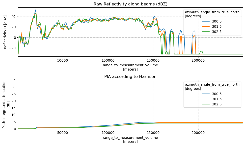
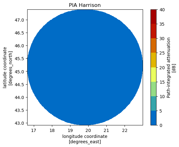
Jacobi & Heistermann (2016) suggested to simply cap PIA in case it would cause a correction of rainfall intensity by more than a factor of two. Depending on the parameters of the Z(R) relationship, that would correspond to PIA values between 4 and 5 dB (4.8 dB if we assume exponent b=1.6).

One way to implement this approach would be the following:

pia_harrison = dbz.wrl.atten.correct_attenuation_hb(coefficients=dict(a=4.57e-5, b=0.731, gate_length=gate_length), mode="warn", thrs=59.0
)
pia_harrison = pia_harrison.clip(max=4.8)

And the results would look like this:

fig, (ax1, ax2) = plt.subplots(2, 1, figsize=(10, 6))
sel = dbz.sel(azimuth=slice(*azi_slice))
sel.plot.line(ax=ax1, hue="azimuth")
ax1.grid(True, which='both', linestyle='--', alpha=0.7)
ax1.set_xlim(float(sel.range.min()), float(sel.range.max()))
ax1.set_title("Raw Reflectivity along beams (dBZ)")
sel2 = pia_harrison.sel(azimuth=slice(*azi_slice))
sel2.plot.line(ax=ax2, hue="azimuth")
ax2.grid(True, which='both', linestyle='--', alpha=0.7)
ax2.set_xlim(float(sel.range.min()), float(sel.range.max()))
ax2.set_ylim(0, 35)
ax2.set_title("PIA according to Harrison")
plt.tight_layout()

corrected signal over threshold (59.0)

pia_harrison.wrl.vis.plot(**pia_kwargs)
plt.gca().set_title("PIA Harrison")

corrected signal over threshold (59.0)

3. Kraemer¶

Krämer & Verworn (2009) suggested to iteratively determine the power law parameters of the A(Z) relation. In particular, the power law coefficient is iteratively decreased until the attenuation correction does not lead to reflectivity values above a given threshold (Kraemer suggested 59 dBZ). Using {{wradlib}}, this would be called by using the function - wradlib.atten.AttenMethods.correct_attenuation_constrained with a specific constraints argument:

pia_kraemer = dbz.wrl.atten.correct_attenuation_constrained(
    a_max=5.0e-5,  # 5.0e-5,
    a_min=2.0e-5,  # 4.0e-5,
    n_a=100,
    b_max=0.75,  # 0.75,
    b_min=0.65,  # 0.71,
    n_b=6,
    gate_length=gate_length,
    constraints=[wrl.atten.constraint_dbz],
    constraint_args=[[59.0]],
)

In brief, this call specifies ranges of the power parameters a and b of the A(Z) relation. Beginning from the maximum values (a_max and b_max), the function searches for values of a and b so that the corrected reflectivity will not exceed the dBZ constraint of 59 dBZ. Compared to the previous results, the corresponding profiles of PIA look like this:

fig, (ax1, ax2) = plt.subplots(2, 1, figsize=(10, 6))
sel = dbz.sel(azimuth=slice(*azi_slice))
sel.plot.line(ax=ax1, hue="azimuth")
ax1.grid(True, which='both', linestyle='--', alpha=0.7)
ax1.set_xlim(float(sel.range.min()), float(sel.range.max()))
ax1.set_title("Raw Reflectivity along beams (dBZ)")
sel2 = pia_kraemer.sel(azimuth=slice(*azi_slice))
sel2.plot.line(ax=ax2, hue="azimuth")
ax2.grid(True, which='both', linestyle='--', alpha=0.7)
ax2.set_xlim(float(sel.range.min()), float(sel.range.max()))
ax2.set_ylim(0, 35)
ax2.set_title("PIA according to Kraemer")
plt.tight_layout()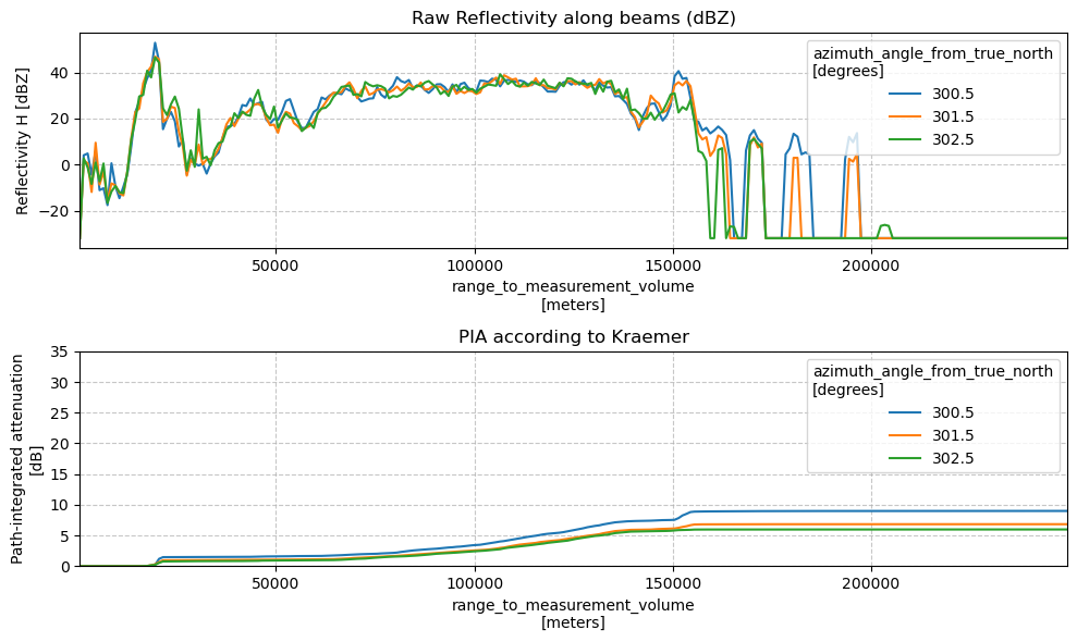

pia_kraemer.wrl.vis.plot(**pia_kwargs)
plt.gca().set_title("PIA Krämer")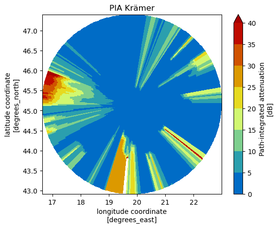

4. Modified Kraemer¶

The function wradlib.atten.AttenMethods.correct_attenuation_constrained allows us to pass any kind of constraint function or lists of constraint functions via the argument constraints. The arguments of these functions are passed via a nested list as argument constraint_args. For example, Jacobi & Heistermann (2016) suggested to constrain both the corrected reflectivity (by a maximum of 59 dBZ) and the resulting path-integrated attenuation PIA (by a maximum of 20 dB):

pia_mkraemer = dbz.wrl.atten.correct_attenuation_constrained(
    a_max=5.0e-5,  # 5.0e-5,
    a_min=2.0e-5,  # 4.0e-5,
    n_a=100,
    b_max=0.75,  # 0.75,
    b_min=0.65,  # 0.71,
    n_b=6,
    gate_length=gate_length,
    constraints=[wrl.atten.constraint_dbz, wrl.atten.constraint_pia],
    constraint_args=[[59.0], [10.0]],
)

fig, (ax1, ax2) = plt.subplots(2, 1, figsize=(10, 6))
sel = dbz.sel(azimuth=slice(*azi_slice))
sel.plot.line(ax=ax1, hue="azimuth")
ax1.grid(True, which='both', linestyle='--', alpha=0.7)
ax1.set_xlim(float(sel.range.min()), float(sel.range.max()))
ax1.set_title("Raw Reflectivity along beams (dBZ)")
sel2 = pia_mkraemer.sel(azimuth=slice(*azi_slice))
sel2.plot.line(ax=ax2, hue="azimuth")
ax2.grid(True, which='both', linestyle='--', alpha=0.7)
ax2.set_xlim(float(sel.range.min()), float(sel.range.max()))
ax2.set_ylim(0, 35)
ax2.set_title("PIA according to modified Kraemer")
plt.tight_layout()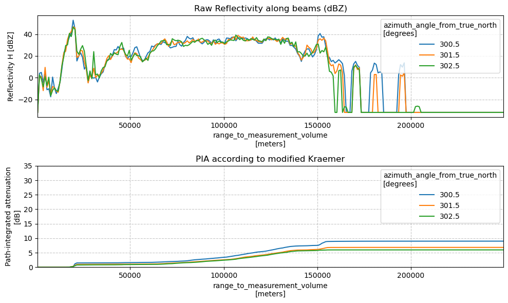

pia_mkraemer.wrl.vis.plot(**pia_kwargs)
plt.gca().set_title("PIA Modified Krämer")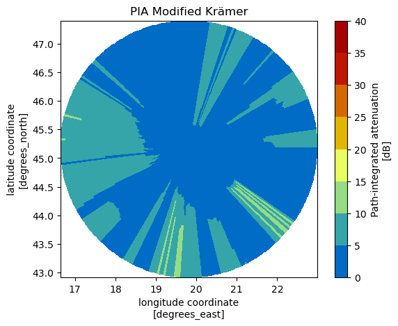

Comparison¶

fig = plt.figure(figsize=(12, 6))
dbz.wrl.vis.plot(ax=121, **dbz_kwargs)
plt.gca().set_title("DBZH")
dbz_corr = dbz + pia_hibo
dbz_corr.attrs = dbz.attrs
dbz_corr.wrl.vis.plot(ax=122, **dbz_kwargs)
plt.gca().set_title("DBZH + PIA")
fig.suptitle("1. Hitschfeld & Bordan", fontsize=16)
fig.tight_layout()

corrected signal over threshold (59.0)

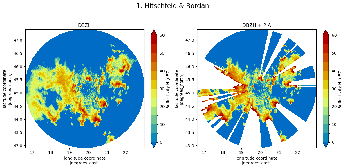
fig = plt.figure(figsize=(12, 6))
dbz.wrl.vis.plot(ax=121, **dbz_kwargs)
plt.gca().set_title("DBZH")
dbz_corr = dbz + pia_harrison
dbz_corr.attrs = dbz.attrs
dbz_corr.wrl.vis.plot(ax=122, **dbz_kwargs)
plt.gca().set_title("DBZH + PIA")
fig.suptitle("2. Harrison", fontsize=16)
fig.tight_layout()

corrected signal over threshold (59.0)

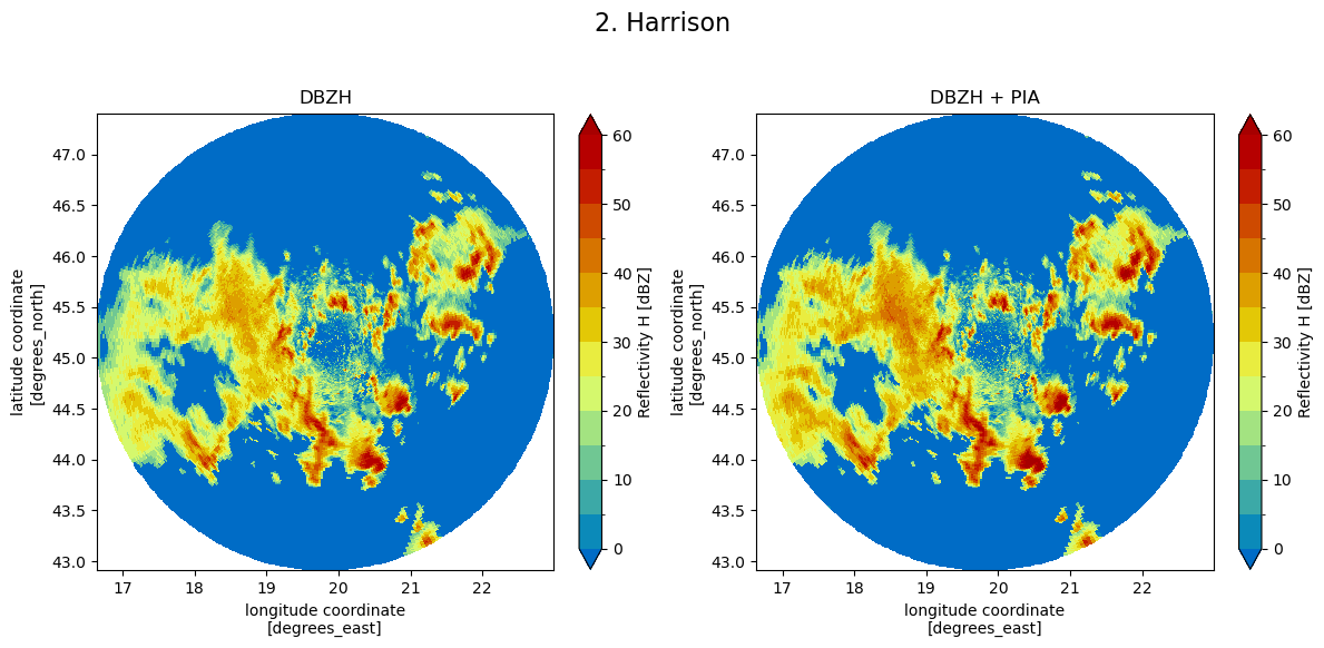
fig = plt.figure(figsize=(12, 6))
dbz.wrl.vis.plot(ax=121, **dbz_kwargs)
plt.gca().set_title("DBZH")
dbz_corr = dbz + pia_kraemer
dbz_corr.attrs = dbz.attrs
dbz_corr.wrl.vis.plot(ax=122, **dbz_kwargs)
plt.gca().set_title("DBZH + PIA")
fig.suptitle("3. Krämer", fontsize=16)
fig.tight_layout()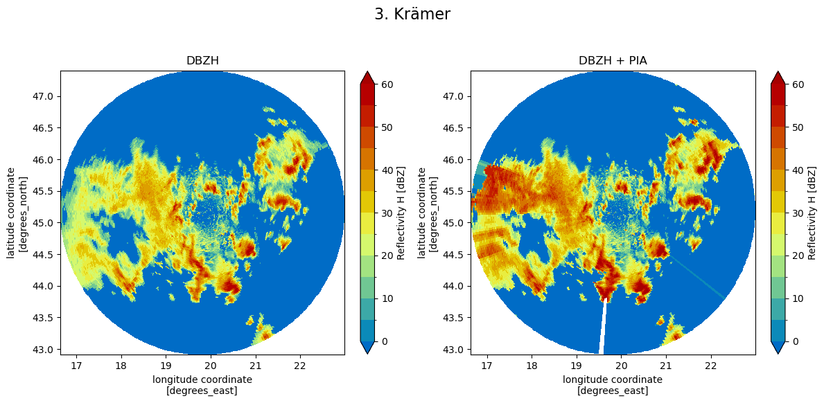

fig = plt.figure(figsize=(12, 6))
dbz.wrl.vis.plot(ax=121, **dbz_kwargs)
plt.gca().set_title("DBZH")
dbz_corr = dbz + pia_mkraemer
dbz_corr.attrs = dbz.attrs
dbz_corr.wrl.vis.plot(ax=122, **dbz_kwargs)
plt.gca().set_title("DBZH + PIA")
fig.suptitle("4. Modified Krämer", fontsize=16)
fig.tight_layout()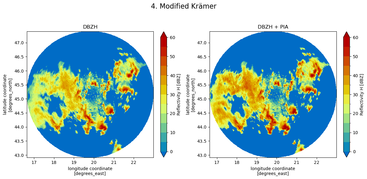

Next Steps¶

You’ve completed the single pol attenuation correction workflow for the selected dataset. Return to Get lowest elevation sweep, select the other case study day, and rerun the notebook.

References¶

Krämer, S., & Verworn, H.-R. (2009). Improved radar data processing algorithms for quantitative rainfall estimation in real time. Water Science and Technology, 60(1), 175–184. 10.2166/wst.2009.282
Jacobi, S., & Heistermann, M. (2016). Benchmarking attenuation correction procedures for six years of single-polarized C-band weather radar observations in South-West Germany. Geomatics, Natural Hazards and Risk, 7(6), 1785–1799. 10.1080/19475705.2016.1155080
Hitschfeld, W., & Bordan, J. (1954). ERRORS INHERENT IN THE RADAR MEASUREMENT OF RAINFALL AT ATTENUATING WAVELENGTHS. Journal of Meteorology, 11(1), 58–67. https://doi.org/10.1175/1520-0469(1954)011<;0058:eiitrm>2.0.co;2