



Quantitative Precipitation Estimation (QPE)
Quantitative Precipitation Estimation converts radar reflectivity into rain rate and, by integrating over time, rainfall accumulation. The Marshall & Palmer Marshall & Palmer (1948) power-law Z-R relationship is the simplest and most widely used approach, and performs best in widespread, layered (stratiform) precipitation where drop-size distributions are relatively uniform — the case used here.
Prerequisites
| Concepts | Importance | Notes |
|---|---|---|
| Xarray Basics | Necessary | Working with radar DataTrees |
| Weather Radar Fundamentals | Helpful | Reflectivity and Z-R relationships |
Time to learn: 15 minutes
Overview
Marshall & Palmer Marshall & Palmer (1948) measured raindrop size distributions in stratiform rain at McGill University and found they closely follow an exponential form,
with roughly constant and decreasing as rain rate increases. Integrating this drop-size distribution to get the radar reflectivity factor (the sixth moment of ) and the rain rate (related to the third moment and fall speed) separately, then eliminating , yields a power-law relationship between the two:
with their now-classic coefficients , ( in , in ). Because these coefficients were fit to a stratiform-rain drop-size distribution, they shouldn’t be assumed to hold in convective rain or snow, where the particle-size distribution differs substantially — other , pairs exist for those regimes, and dual-polarization estimators such as R(KDP) are more robust in heavy rain since they are insensitive to attenuation and less sensitive to drop-size assumptions — see Attenuation correction - Dual Pol.
We use the single-polarization Fruška Gora data here (rather than the dual-polarization Jastrebac data used for the convective QVP) paired with the stratiform case (Stratiform Case 2014): a single Z-R relationship is best justified over a widespread, more uniform rain event than a convective one.
Claim Data
We use the ARCO data provided in Data Access — Serbian Rainbow Radar.
OSN_ENDPOINT = "https://umn1.osn.mghpcc.org"
BUCKET = "nexrad-arco"
prefix = "Fgora" # single-pol, 12 sweeps × 360 az × 250 range, 2014 + 2017 + 2026 — stratiform case
storage = icechunk.s3_storage(
bucket=BUCKET,
prefix=prefix,
endpoint_url=OSN_ENDPOINT,
region="us-east-1",
anonymous=True,
force_path_style=True,
)
repo = icechunk.Repository.open(storage)
dtree = xr.open_datatree(
repo.readonly_session("main").store,
engine="zarr",
consolidated=False,
chunks={},
).sel(vcp_time="2014")
display(dtree)
root = next(iter(dtree.keys())).split("/")[0]Get the Lowest Elevation Sweep
QPE conventionally uses the lowest available elevation, closest to the ground, to minimize the vertical distance between the radar beam and the surface.
swp = (
    dtree[f"{root}/sweep_0"]
    .to_dataset(inherit="all_coords")
    .wrl.georef.georeference(crs=wrl.georef.get_earth_projection())
)
swp.z.attrs = xd.model.get_altitude_attrs()
display(swp)Convert Reflectivity to Rain Rate
z_linear = swp.DBZH.wrl.trafo.idecibel()
rain_rate = z_linear.wrl.zr.z_to_r(a=200.0, b=1.6)
rain_rate.attrs.update(units="mm/h", long_name="Rain rate (Marshall-Palmer)")
display(rain_rate)Accumulate Rainfall
We convert each scan’s instantaneous rain rate into a rainfall depth using the volume’s median scan interval, then sum over the full period to get total accumulation.
dt_minutes = float(np.median(np.diff(swp.vcp_time.values)) / np.timedelta64(1, "m"))
print(f"Median scan interval: {dt_minutes:.1f} minutes")

accumulation = (rain_rate * dt_minutes / 60.0).sum("vcp_time", skipna=True)
accumulation.name = "accum"
accumulation.attrs.update(units="mm", long_name="Rainfall accumulation")
display(accumulation)
Median scan interval: 5.0 minutes
Visualize Accumulated Rainfall
fig = plt.figure(figsize=(8, 7))
accumulation.wrl.vis.plot(cmap="HomeyerRainbow", vmin=0, vmax=15)
plt.gca().set_title(f"{prefix} - Rainfall Accumulation")
fig.tight_layout()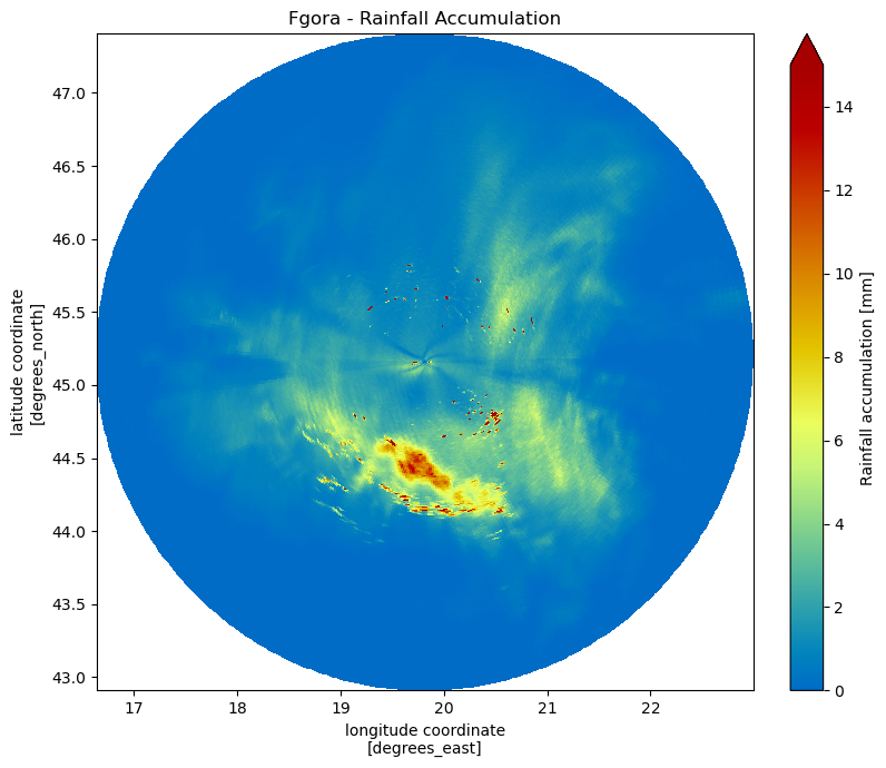
Next Steps
You’ve computed a single Z-R rainfall accumulation for the stratiform case. Return to the prefix selection step to try one of the other Fruška Gora dates.
- Marshall, J. S., & Palmer, W. M. K. (1948). THE DISTRIBUTION OF RAINDROPS WITH SIZE. Journal of Meteorology, 5(4), 165–166. https://doi.org/10.1175/1520-0469(1948)005<;0165:tdorws>2.0.co;2