Terrain and Beam Blockage¶

Prerequisites¶

Concepts	Importance	Notes
Xarray Basics	Helpful	Working with radar and DEM datasets
Raster Data Fundamentals	Helpful	Digital elevation models and georeferenced rasters
GDAL Basics	Helpful	Raster mosaicking and reprojection
Weather Radar Geometry	Helpful	Radar coordinates, beam propagation, and beam blockage

Time to learn: 15 minutes

Overview¶

In this notebook, we demonstrate a terrain-aware radar processing workflow using wradlib and the scientific Python ecosystem. Radar data are read directly from cloud storage using Xarray, while digital elevation data are retrieved from publicly available SRTM tiles. The individual DEM tiles are merged into a seamless raster, interpolated onto the radar grid, and used to compute partial and cumulative beam blockage following Bech et al. The resulting products provide insight into the influence of terrain on radar observations.

Imports¶

import numpy as np
import wradlib as wrl
import matplotlib.pyplot as plt
import xarray as xr
import xradar as xd
import fsspec
import icechunk
from pathlib import Path
import warnings
warnings.filterwarnings("ignore", category=RuntimeWarning)

Claim Data¶

The examples in this notebook can be run with different radar datasets. Select the desired dataset by setting the prefix variable below. The available options include a single-polarization volume from Fruška Gora (fgora_vol) and dual-polarization volumes from Jastrebac at different range resolutions (jastrebac_250m and jastrebac_500m). All subsequent processing steps will automatically use the selected dataset.

OSN_ENDPOINT = "https://umn1.osn.mghpcc.org"
BUCKET = "nexrad-arco"

# prefix = "Fgora"  # single-pol, 12 sweeps × 360 az × 250 range, 2014 + 2017 + 2026
prefix = "jastrebac_250m"  # dual-pol, 12 × 360 × 1000, 2014 only
# prefix = "jastrebac_500m"  # dual-pol, 12 × 360 × 500,  2017 + 2026

print(f"Using prefix {prefix}")

Using prefix jastrebac_250m

storage = icechunk.s3_storage(
    bucket=BUCKET,
    prefix=prefix,
    endpoint_url=OSN_ENDPOINT,
    region="us-east-1",
    anonymous=True,
    force_path_style=True,
)
repo = icechunk.Repository.open(storage)
dtree = xr.open_datatree(
    repo.readonly_session("main").store,
    engine="zarr",
    consolidated=False,
    chunks={},
)
display(dtree)
root = next(iter(dtree.keys())).split("/")[0]

Get sweep¶

sweep = "sweep_0"

swp = (
    dtree[f"{root}/{sweep}"]
    .to_dataset()
    .assign_coords(dtree[root].coords)
    .assign_coords(sweep_mode="azimuth_surveillance")
    .wrl.georef.georeference(crs=wrl.georef.get_earth_projection())
)
swp.x.attrs = xd.model.get_longitude_attrs()
swp.y.attrs = xd.model.get_latitude_attrs()
swp.z.attrs = xd.model.get_altitude_attrs()

Digital Elevation Map (DEM)¶

Elevation data were derived from the NASA Shuttle Radar Topography Mission (Farr & Kobrick (2000), Farr et al. (2007), SRTMGL3 v003, 3 arc-second resolution) and are accessed via the Terrain Tiles (Mapzen / AWS Open Data Registry). distribution (Skadi format). The dataset is based on SRTM global elevation measurements provided by NASA JPL (2013) and distributed through NASA LP DAAC.

Download DEM¶

We retrieve the required SRTM elevation tiles from the public AWS Terrain Tiles (Skadi) S3 bucket. The tiles are selected based on the spatial extent of the study area and downloaded locally for further processing.

The individual DEM tiles are merged into a single seamless raster using GDAL. This step leverages GDAL’s efficient raster warping and mosaicking capabilities while preserving georeferencing information.

The merged DEM is opened using Rasterio and exposed as an Xarray dataset. This provides labeled coordinates and enables convenient analysis and integration with downstream geospatial workflows.

from pathlib import Path
import requests
from requests.adapters import HTTPAdapter
from urllib3.util.retry import Retry

BASE = "https://elevation-tiles-prod.s3.amazonaws.com"

session = requests.Session()

retry = Retry(
    total=6,
    backoff_factor=1.5,
    status_forcelist=[500, 502, 503, 504],
    allowed_methods=["GET"],
    raise_on_status=False,
)

session.mount("https://", HTTPAdapter(max_retries=retry))

def download_skadi_tile(tile, destination=None):
    destination = Path(destination or f"{tile}.hgt.gz")

    if destination.exists():
        return destination

    key = f"skadi/{tile[:3]}/{tile}.hgt.gz"
    url = f"{BASE}/{key}"

    print(f"Downloading {url}")

    with session.get(url, stream=True, timeout=60) as r:
        r.raise_for_status()
        with destination.open("wb") as f:
            for chunk in r.iter_content(1024 * 1024):
                if chunk:
                    f.write(chunk)

    return destination

extent = [swp.x.min().values, swp.x.max().values, swp.y.min().values, swp.y.max().values]
tiles = wrl.io.dem.get_srtm_tile_names(extent)
tiles = [f"/vsigzip/{download_skadi_tile(tile)}" for tile in tiles]

drm_file = wrl.io.merge_srtm(tiles, destination=f"{prefix}.tif")
print(drm_file)

jastrebac_250m.tif

dem = (
    xr.open_dataset(drm_file, engine="rasterio", chunks={"x": -1, "y": -1})
    .isel(band=0)
    .rename(band_data="DEM")
    .reset_coords("band", drop=True)
).chunk(x=500, y=500)
display(dem)

Prepare DEM¶

We interpolate the raster DEM onto the polar radar grid so that each radar gate is assigned a corresponding elevation value. The resulting DEM layer is then added to the radar sweep dataset, enabling joint analysis of radar measurements and terrain information.

dem_polar = dem.DEM.chunk(x=-1, y=-1).wrl.ipol.interpolate(swp.isel(vcp_time=0, range=slice(0, 1000)), method="map_coordinates", order=1)
display(dem_polar)
swp = swp.assign(DEM=dem_polar)

swp.DEM.wrl.vis.plot(vmin=0, cmap="terrain")
plt.gca().set_title("DEM - Polar Radar Grid")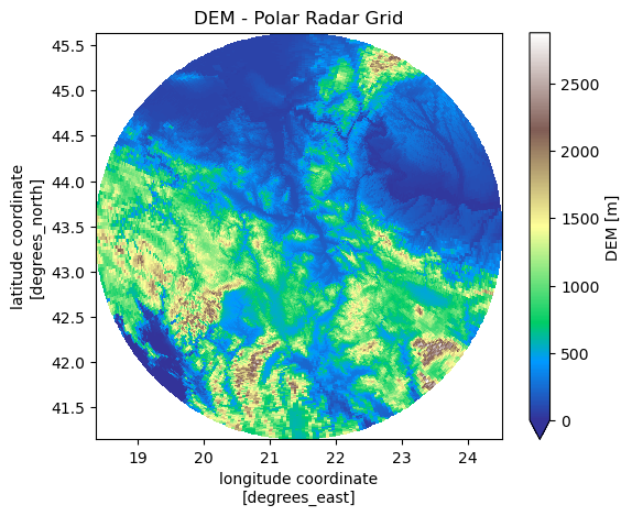

BeamBlockage Calculation¶

We compute partial beam blockage (PBB) and cumulative beam blockage (CBB) using the interpolated DEM in radar sweep coordinates. Following Bech et al. (2003), the terrain influence on the radar beam is quantified by estimating how much of the beam is obstructed along each radial path, first as a local (partial) blockage fraction and then accumulated along the beam path.

bw = 0.9
PBB = swp.DEM.wrl.qual.beam_block_frac(bw)
CBB = PBB.wrl.qual.cum_beam_block_frac()
swp = swp.assign(
    CBB=CBB,
    PBB=PBB,
)

fig = swp.wrl.vis.plot_beamblockage(angle=255., ylim=(0, 10000))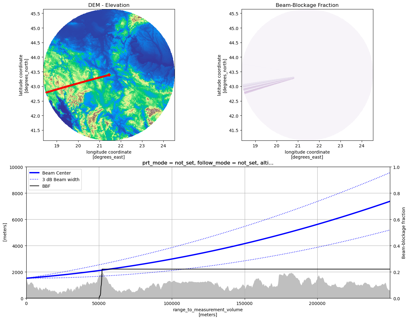

Write DEM and Beamblockage¶

To avoid repeatedly downloading and processing the radar volume and raster data, we store the selected output as a NetCDF file. This allows subsequent analyses to be performed directly from the local file while preserving the full dataset structure and metadata. prefix and sweep are encoded in the file name.

outdir = Path.cwd()
outname = f"{prefix}_{sweep}_dem.nc"
swp[["DEM", "PBB", "CBB"]].to_netcdf(outdir / outname)

dem_bb = xr.open_dataset(outname)
print(outname)
display(dem_bb)

jastrebac_250m_sweep_0_dem.nc

Next Steps¶

You’ve finished processing the selected dataset. Return to prefix selection step, choose one of the remaining datasets, and rerun the notebook. Repeat this until all three datasets have been processed.

References¶

Farr, T. G., & Kobrick, M. (2000). Shuttle radar topography mission produces a wealth of data. Eos, Transactions American Geophysical Union, 81(48), 583–585. 10.1029/eo081i048p00583
Farr, T. G., Rosen, P. A., Caro, E., Crippen, R., Duren, R., Hensley, S., Kobrick, M., Paller, M., Rodriguez, E., Roth, L., Seal, D., Shaffer, S., Shimada, J., Umland, J., Werner, M., Oskin, M., Burbank, D., & Alsdorf, D. (2007). The Shuttle Radar Topography Mission. Reviews of Geophysics, 45(2). 10.1029/2005rg000183
NASA JPL. (2013). NASA Shuttle Radar Topography Mission Global 3 arc second. NASA Land Processes Distributed Active Archive Center. 10.5067/MEASURES/SRTM/SRTMGL3.003
Bech, J., Codina, B., Lorente, J., & Bebbington, D. (2003). The Sensitivity of Single Polarization Weather Radar Beam Blockage Correction to Variability in the Vertical Refractivity Gradient. Journal of Atmospheric and Oceanic Technology, 20(6), 845–855. https://doi.org/10.1175/1520-0426(2003)020<;0845:tsospw>2.0.co;2