System Differential Phase¶

Correct retrieval of System Differential Phase $\Phi_{DP}^{sys}$ (aka system offset) is crucial for the accurate processing of all derived polarimetric products. In general, $\Phi_{DP}^{sys}$ is assumed to be constant. However, it may exhibit azimuthal or elevational variations, for example due to antenna near-field effects.

Retrieval of $\Phi_{DP}^{sys}$ is sometimes tedious, due to the contamination of the signal with clutter and other artifacts.

Import Section¶

import cmweather
import numpy as np
import matplotlib.pyplot as plt
import wradlib as wrl
import xarray as xr
import xradar as xd
import fsspec
import icechunk
import holoviews as hv
import hvplot
import hvplot.xarray
import warnings
warnings.filterwarnings("ignore")

Claim Data¶

We use the ARCO data provided in Data Access — Serbian Rainbow Radar. Please refer to this notebook for details of access.

OSN_ENDPOINT = "https://umn1.osn.mghpcc.org"
BUCKET = "nexrad-arco"

prefix = "jastrebac_250m"  # dual-pol, 12 × 360 × 1000, 2014 only
# prefix = "jastrebac_500m"  # dual-pol, 12 × 360 × 500,  2017 + 2026

storage = icechunk.s3_storage(
    bucket=BUCKET,
    prefix=prefix,
    endpoint_url=OSN_ENDPOINT,
    region="us-east-1",
    anonymous=True,
    force_path_style=True,
)
repo = icechunk.Repository.open(storage)
dtree = xr.open_datatree(
    repo.readonly_session("main").store,
    engine="zarr",
    consolidated=False,
    chunks={},
)
display(dtree)
root = next(iter(dtree.keys())).split("/")[0]

Get lowest elevation sweep¶

First we get the lowest sweep and do some georeferencing.

swp = (
    dtree[f"{root}/sweep_0"]
    .to_dataset()
    .assign_coords(dtree[root].coords)
    .assign_coords(sweep_mode="azimuth_surveillance")
    .wrl.georef.georeference(crs=wrl.georef.get_earth_projection())
).sel(vcp_time="2014")
swp.x.attrs = xd.model.get_longitude_attrs()
swp.y.attrs = xd.model.get_latitude_attrs()
swp.z.attrs = xd.model.get_altitude_attrs()
display(swp)

Inspect Dataset¶

display(swp)

fig, (ax1, ax2) = plt.subplots(1, 2, figsize=(12, 8), sharey=True)
swp.uPhiDP[0].wrl.vis.plot(ax=ax1, vmin=0, vmax=360)
ax1.set_title("Raw uPhiDP")
swp.PHIDP[0].wrl.vis.plot(ax=ax2, vmin=0, vmax=360)
ax2.set_title("Raw PHIDP (preprocessed)")
fig.tight_layout()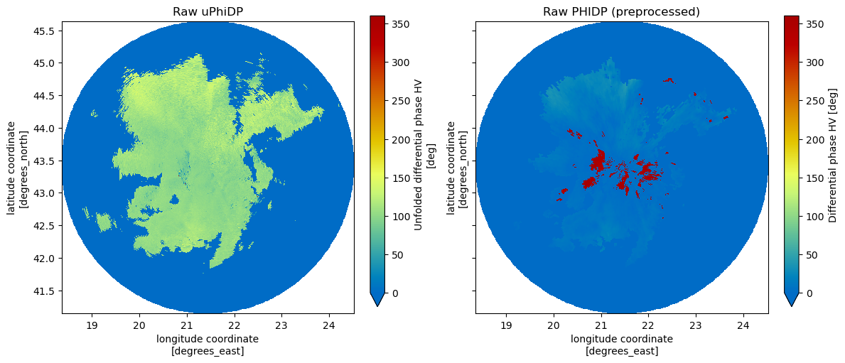

System Differential Phase $\Phi_{DP}^{sys}$ via first precipitating bins¶

This is a most common algorithm. But there are several approaches. All use common $\rho_{HV}$ filtering or other means of reducing unwanted artifacts in $\Phi_{DP}^{sys}$ .

N consecutive radar bins with $\rho_{HV}$ > threshold
first N valid bins with $\rho_{HV}$ > threshold (not necessarily consecutive)

Mask source data¶

Essential pre-step masking unwanted signal.

phimask = swp.uPhiDP.where(swp.RHOHV >= 0.9)

N consecutive valid radar bins¶

It finds the first N consecutive precipitating bins per each ray
and uses the median of these values to determine the offset per ray.
If there are only a few of those radials (<30) per sweep we’ll use a default value from a previous sweep
Sort the median values from 2. and calculate the median from the smallest 30 (default).

That value is considered $\Phi_{DP}^{sys}$ .

phisys_block = phimask.wrl.dp.system_phidp_block(rng=2000.)
display(phisys_block)

vcp = 0

fig, (ax1, ax2) = plt.subplots(2, 1, figsize=(10, 10), sharex=True)
phisys_block.isel(vcp_time=vcp).start_range.plot(ax=ax1, lw=0.8, c="k")
phisys_block.isel(vcp_time=vcp).stop_range.plot(ax=ax1, lw=0.8, c="k")
phimask.isel(vcp_time=vcp).plot(ax=ax1, x="azimuth", y="range", cmap="turbo", vmin=0, vmax=140)
ax1.set_title(rf"$\phi_{{DP}}^{{sys}}$ - {phisys_block.isel(vcp_time=vcp).valid_bins[0].values} consecutive valid radar bins")

phisys_block.isel(vcp_time=vcp).start_range.plot(ax=ax2, lw=0.8, c="k")
phisys_block.isel(vcp_time=vcp).stop_range.plot(ax=ax2, lw=0.8, c="k")
phimask.isel(vcp_time=vcp).plot(ax=ax2, x="azimuth", y="range", cmap="turbo", vmin=0, vmax=140)
ax2.set_title(rf"$\phi_{{DP}}^{{sys}}$ - zoom")
ax2.set_ylim(0, 15e3)
display(phisys_block.sysphi)
fig.tight_layout()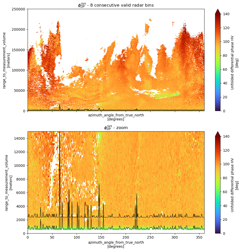

fig = plt.figure()
ax = fig.add_subplot(projection="polar")
# set the lable go clockwise and start from the top
ax.set_theta_zero_location("N")
# clockwise
ax.set_theta_direction(-1)

theta = np.linspace(0, 2 * np.pi, num=phisys_block.dims["azimuth"], endpoint=False)
ax.plot(theta, phisys_block.isel(vcp_time=vcp).sysphi_ray, color="b", linewidth=1)
ax.plot(theta, np.ones_like(theta)*phisys_block.isel(vcp_time=vcp).sysphi.values, color="r", linewidth=1)
_ = ax.set_title(rf"$\phi_{{DP}}^{{sys}}$ - {phisys_block.isel(vcp_time=vcp).sysphi.values} deg")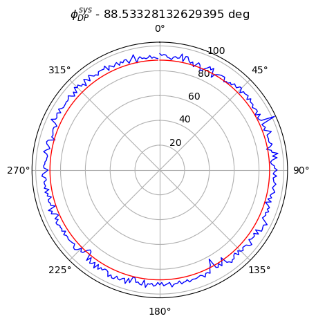

first N valid bins¶

Get the first N valid bins per each ray
Calculate median from these values
Sort the median values from 2. and calculate the median from the smallest 30.

That value is considered $\Phi_{DP}^{sys}$ .

phisys_first = phimask.wrl.dp.system_phidp_first(11)
display(phisys_first)

fig, (ax1, ax2) = plt.subplots(2, 1, figsize=(10, 10), sharex=True)
phisys_first.isel(vcp_time=vcp).start_range.plot(ax=ax1, lw=0.8, c="k")
phisys_first.isel(vcp_time=vcp).stop_range.plot(ax=ax1, lw=0.8, c="k")
phimask.isel(vcp_time=vcp).plot(ax=ax1, x="azimuth", y="range", cmap="turbo", vmin=0, vmax=140)
ax1.set_title(rf"$\phi_{{DP}}^{{sys}}$ - {phisys_first.isel(vcp_time=vcp).valid_bins[0].values} valid radar bins")

phisys_first.isel(vcp_time=vcp).start_range.plot(ax=ax2, lw=0.8, c="k")
phisys_first.isel(vcp_time=vcp).stop_range.plot(ax=ax2, lw=0.8, c="k")
phimask.isel(vcp_time=vcp).plot(ax=ax2, x="azimuth", y="range", cmap="turbo", vmin=0, vmax=140)
ax2.set_title(rf"$\phi_{{DP}}^{{sys}}$ - zoom")
ax2.set_ylim(0, 15e3)
display(phisys_first.isel(vcp_time=vcp).sysphi)
fig.tight_layout()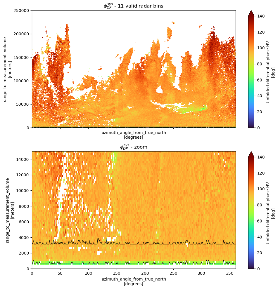

fig = plt.figure()
ax = fig.add_subplot(projection="polar")
# set the lable go clockwise and start from the top
ax.set_theta_zero_location("N")
# clockwise
ax.set_theta_direction(-1)

theta = np.linspace(0, 2 * np.pi, num=phisys_first.dims["azimuth"], endpoint=False)
ax.plot(theta, phisys_first.isel(vcp_time=vcp).sysphi_ray, color="b", linewidth=1)
ax.plot(theta, np.ones_like(theta)*phisys_first.isel(vcp_time=vcp).sysphi.values, color="r", linewidth=1)
_ = ax.set_title(rf"$\phi_{{DP}}^{{sys}}$  - {phisys_first.isel(vcp_time=vcp).sysphi.values} deg")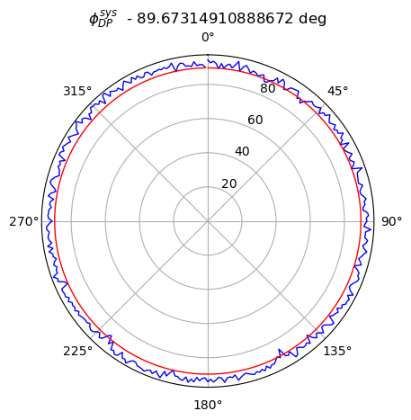

System Differential Phase $\Phi_{DP}^{sys}$ via phase histogram¶

The idea behind is:

$\Phi_{DP}^{sys}$ is constantly increasing
$\Phi_{DP}^{sys}$ is inherently noisy

That means, the majority of phase measurements (precipitating bins) should lie around $\Phi_{DP}^{sys}$ . It’s relatively robust since it does not rely on finding precipitating bins in each ray or the like. Nevertheless, taking a pre-filtered phase as input should return similar results.

from xhistogram.xarray import histogram as xhist

hlist = []
phase_res = 0.1
bins = (0, 360, phase_res)

phisys_hist = swp.uPhiDP.wrl.dp.system_phidp_hist(bins=bins)
phisys_hist_mask = phimask.wrl.dp.system_phidp_hist(bins=bins)
display(phisys_hist)

phisys_hist_s = phisys_hist.isel(vcp_time=vcp)
phisys_hist_s.sysphi_hist.sum("azimuth").rolling(bin=5).mean().plot(label="raw")
phisys_hist_mask_s = phisys_hist_mask.isel(vcp_time=vcp)
phisys_hist_mask_s.sysphi_hist.sum("azimuth").rolling(bin=5).mean().plot(label="masked")
print(phisys_hist_s.sysphi_first.values, phisys_hist_mask_s.sysphi_first.values)
plt.legend()
plt.grid()

91.35000000000001 91.4

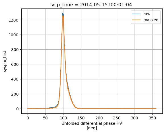
phisys_hist_s.sysphi_hist.sum("azimuth").rolling(bin=5).mean().plot(label="raw")
phisys_hist_mask_s.sysphi_hist.sum("azimuth").rolling(bin=5).mean().plot(label="masked")
plt.gca().set_xlim(0, 100)
plt.gca().set_ylim(0, 100)
plt.legend()
plt.grid()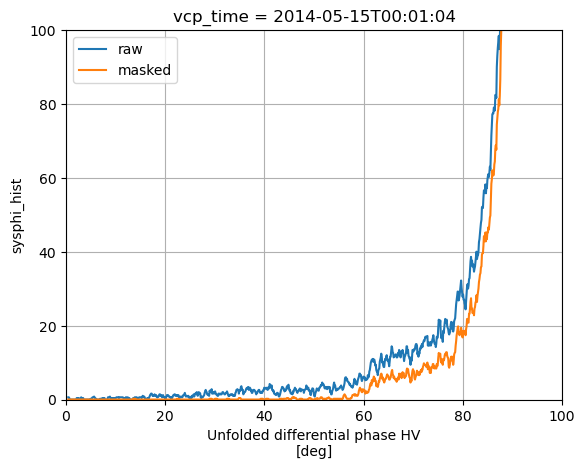

fig = plt.figure()
ax = fig.add_subplot(projection="polar")
# set the lable go clockwise and start from the top
ax.set_theta_zero_location("N")
# clockwise
ax.set_theta_direction(-1)

theta = np.linspace(0, 2 * np.pi, num=phisys_first.dims["azimuth"], endpoint=False)
ax.plot(theta, phisys_hist_s.sysphi_peak_ray, color="b", linewidth=1)
ax.plot(theta, phisys_hist_s.sysphi_first_ray, color="r", linewidth=1)
ax.plot(theta, np.ones_like(theta)*phisys_hist_s.sysphi_peak.values, color="b", linewidth=1.0)
ax.plot(theta, np.ones_like(theta)*phisys_hist_s.sysphi_first.values, color="r", linewidth=1.0)
_ = ax.set_title(rf"$\phi_{{DP}}^{{sys}}$  - {phisys_hist_s.sysphi_first.values} deg")
print(phisys_hist_s.sysphi_peak.values)
ax.set_ylim(60, 100)

95.60000000000001

(60.0, 100.0)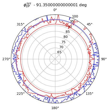

Overview and Diagnostic plots¶

add theta in radians to dataset

theta = np.linspace(0, 2 * np.pi, num=360, endpoint=False)
phisys_block = phisys_block.assign_coords(
    theta=(["azimuth"], theta, {"standard_name": "azimuth angle"})
)
phisys_first = phisys_first.assign_coords(
    theta=(["azimuth"], theta, {"standard_name": "azimuth angle"})
)
phisys_hist_s = phisys_hist_s.assign_coords(
    theta=(["azimuth"], theta, {"standard_name": "azimuth angle"})
)

vmin = 0
vmax = 120
startaz = swp.isel(vcp_time=vcp).sortby("time").azimuth[0]

fig = plt.figure(figsize=(10, 10))
ax = fig.add_subplot(projection="polar")
ax.set_theta_zero_location("N")
ax.set_theta_direction(-1)

ax.axvline(np.radians(startaz.values), c="black", lw=1.0)
phisys_block.isel(vcp_time=vcp).sysphi_ray.plot(x="theta", c="k", lw=0.5, ax=ax)
phisys_first.isel(vcp_time=vcp).sysphi_ray.plot(x="theta", c="r", lw=0.5, ax=ax)
phisys_hist_s.sysphi_peak_ray.plot(x="theta", c="b", lw=0.5, ax=ax)
phisys_hist_s.sysphi_first_ray.plot(x="theta", c="b", lw=0.5, ax=ax)
ax.axhline(phisys_block.isel(vcp_time=vcp).sysphi, c="k").get_path()._interpolation_steps = 180
ax.axhline(phisys_first.isel(vcp_time=vcp).sysphi, c="r").get_path()._interpolation_steps = 180
ax.axhline(phisys_hist_s.sysphi_peak, c="b", ls="--").get_path()._interpolation_steps = 180
ax.axhline(phisys_hist_s.sysphi_first, c="b", ls=":").get_path()._interpolation_steps = 180
ax.set_ylim(vmin, vmax)
ax.set_title(rf"$\phi_{{DP}}^{{sys}}$")
plt.tight_layout()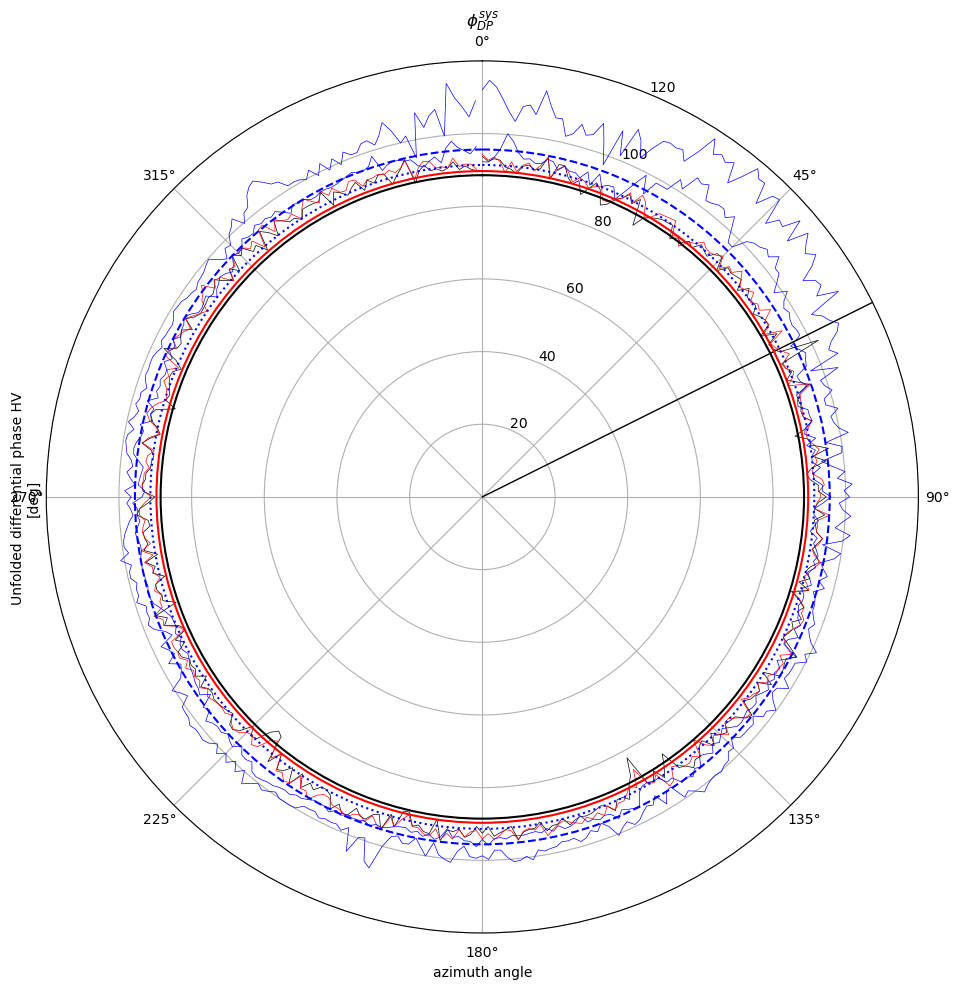

Uncorrected vs corrected $\Phi_{DP}$ ¶

phi_sys = float(phisys_block.isel(vcp_time=vcp).sysphi.compute())

fig = plt.figure(figsize=(14, 12))
swp.uPhiDP.isel(vcp_time=vcp).wrl.vis.plot(ax=221)
plt.gca().set_title("raw uPHIDP") 
swp.uPhiDP.isel(vcp_time=vcp).wrl.vis.plot(ax=222, vmin=phi_sys, vmax=phi_sys+100)
plt.gca().set_title("raw uPHIDP in $\Phi_{DP}^{sys}$ range")
swp.PHIDP.isel(vcp_time=vcp).wrl.vis.plot(ax=223, vmin=0, vmax=100)
plt.gca().set_title("raw PHIDP (pre-corrected)")
phicorr = (swp.uPhiDP.isel(vcp_time=vcp) - phi_sys) 
phicorr.where(phicorr>=0).wrl.vis.plot(ax=224, vmin=0, vmax=100)
plt.gca().set_title("uPHIDP (offset-corrected)")
fig.tight_layout()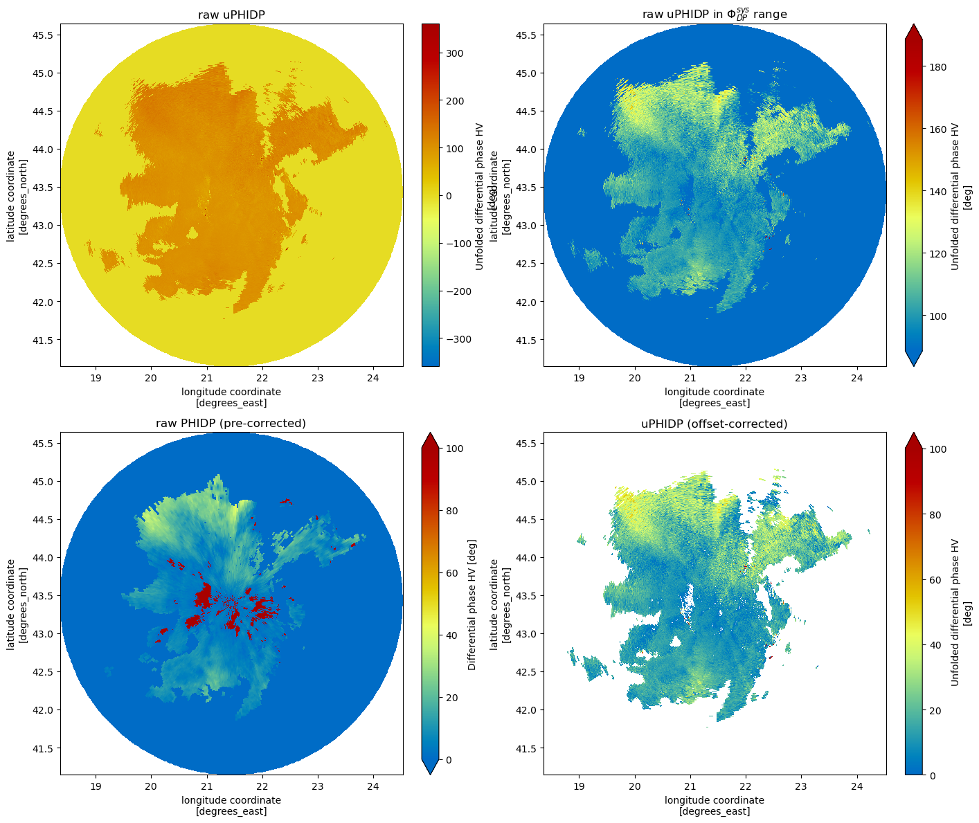

Difference pre-corrected vs corrected $\Phi_{DP}$ ¶

fig = plt.figure(figsize=(14, 12))
precorr = swp.PHIDP.isel(vcp_time=vcp) 
precorr.wrl.vis.plot(ax=221, vmin=0, vmax=100)
plt.gca().set_title("raw PHIDP (pre-corrected)")
phicorr = (swp.uPhiDP.isel(vcp_time=vcp) - phisys_block.isel(vcp_time=vcp).sysphi) 
phicorr.where(phicorr>=0).wrl.vis.plot(ax=222, vmin=0, vmax=100)
plt.gca().set_title("uPHIDP (offset-corrected)")
(precorr - phicorr).where(phicorr>=0).wrl.vis.plot(ax=223, vmin=-10, vmax=10)
plt.gca().set_title("PHIDP - uPhiDP_corr")
fig.tight_layout()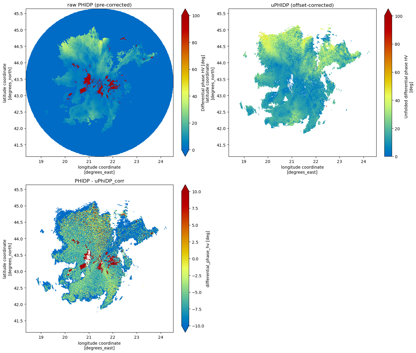

Next Steps¶

You’ve completed the system differential phase offset workflow for the selected dataset. Return to Claim Data, select the other case study day, and rerun the notebook.

You might also save your computed data to disk for later processing.

System Differential Phase

System Differential Phase¶

Import Section¶

Claim Data¶

Get lowest elevation sweep¶

Inspect Dataset¶

System Differential Phase ΦDPsys\Phi_{DP}^{sys}ΦDPsys​ via first precipitating bins¶

Mask source data¶

N consecutive valid radar bins¶

first N valid bins¶

System Differential Phase ΦDPsys\Phi_{DP}^{sys}ΦDPsys​ via phase histogram¶

Overview and Diagnostic plots¶

Uncorrected vs corrected ΦDP\Phi_{DP}ΦDP​¶

Difference pre-corrected vs corrected ΦDP\Phi_{DP}ΦDP​¶

Next Steps¶

System Differential Phase $\Phi_{DP}^{sys}$ via first precipitating bins¶

System Differential Phase $\Phi_{DP}^{sys}$ via phase histogram¶

Uncorrected vs corrected $\Phi_{DP}$ ¶

Difference pre-corrected vs corrected $\Phi_{DP}$ ¶