Differential Phase¶

In this notebook differential phase $\Phi_{DP}$ processing is highlighted. This includes phase unfolding as well as derivation of specific differential phase $K_{DP}$ .

import cmweather
import numpy as np
import matplotlib.pyplot as plt
import wradlib as wrl
import xarray as xr
import xradar as xd
import fsspec
import icechunk
import holoviews as hv
import hvplot
import hvplot.xarray
import warnings
warnings.filterwarnings("ignore")

Claim Data¶

We use the ARCO data provided in Data Access — Serbian Rainbow Radar. Please refer to this notebook for details of access.

OSN_ENDPOINT = "https://umn1.osn.mghpcc.org"
BUCKET = "nexrad-arco"

prefix = "jastrebac_250m"  # dual-pol, 12 × 360 × 1000, 2014 only
# prefix = "jastrebac_500m"  # dual-pol, 12 × 360 × 500,  2017 + 2026

storage = icechunk.s3_storage(
    bucket=BUCKET,
    prefix=prefix,
    endpoint_url=OSN_ENDPOINT,
    region="us-east-1",
    anonymous=True,
    force_path_style=True,
)
repo = icechunk.Repository.open(storage)
dtree = xr.open_datatree(
    repo.readonly_session("main").store,
    engine="zarr",
    consolidated=False,
    chunks={},
)
display(dtree)
root = next(iter(dtree.keys())).split("/")[0]

Get lowest elevation sweep¶

First we get the lowest sweep and do some georeferencing.

swp = (
    dtree[f"{root}/sweep_0"]
    .to_dataset()
    .assign_coords(dtree[root].coords)
    .assign_coords(sweep_mode="azimuth_surveillance")
    .wrl.georef.georeference(crs=wrl.georef.get_earth_projection())
).sel(vcp_time="2014")
swp.x.attrs = xd.model.get_longitude_attrs()
swp.y.attrs = xd.model.get_latitude_attrs()
swp.z.attrs = xd.model.get_altitude_attrs()
display(swp)

Mask with RHOHV¶

First, we mask with $\rho_{HV}$ and/or any other moment you trust to remove unwanted signal.

mask = (swp.RHOHV >= 0.9)
mswp = swp.where(mask)

Second, we estimate system differential phase offset $\Phi_{DP}^{sys}$ , see System Differential Phase Notebook for details.

phase_res = 0.1
bins = (0, 360, phase_res)
phisys_hist = mswp.uPhiDP.wrl.dp.system_phidp_hist(bins=bins)
display(phisys_hist)
phisys_hist.sysphi_peak.plot()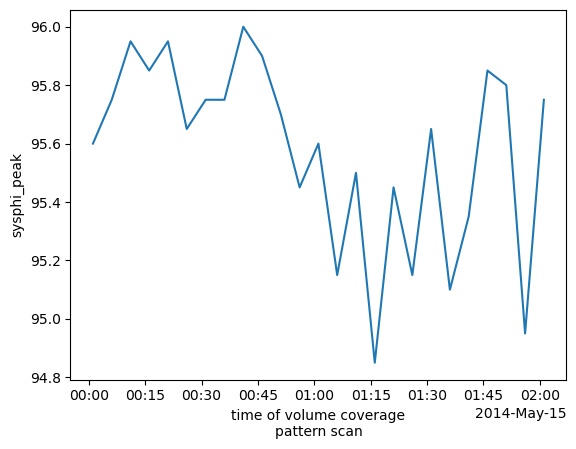

Overview Plots¶

Let’s have a look how the provided raw $\Phi_{DP}$ and $K_{DP}$ look like. In the dataset the uncorrected $\Phi_{DP}$ uPhiDP is provided as well as the pre-corrected PHIDP (which has some issues).

Select vcp_time index¶

vcp = 0
system_offset = phisys_hist.isel(vcp_time=vcp).sysphi_peak.values

Unmasked RAW¶

fig, (ax1, ax2) = plt.subplots(1, 2, figsize=(12, 5))
swp.uPhiDP.isel(vcp_time=vcp).wrl.vis.plot(ax=ax1)
ax1.set_title("Raw $\Phi_{DP}$")
swp.KDP.isel(vcp_time=vcp).wrl.vis.plot(ax=ax2)
ax2.set_title("Raw $K_{DP}$")
fig.tight_layout()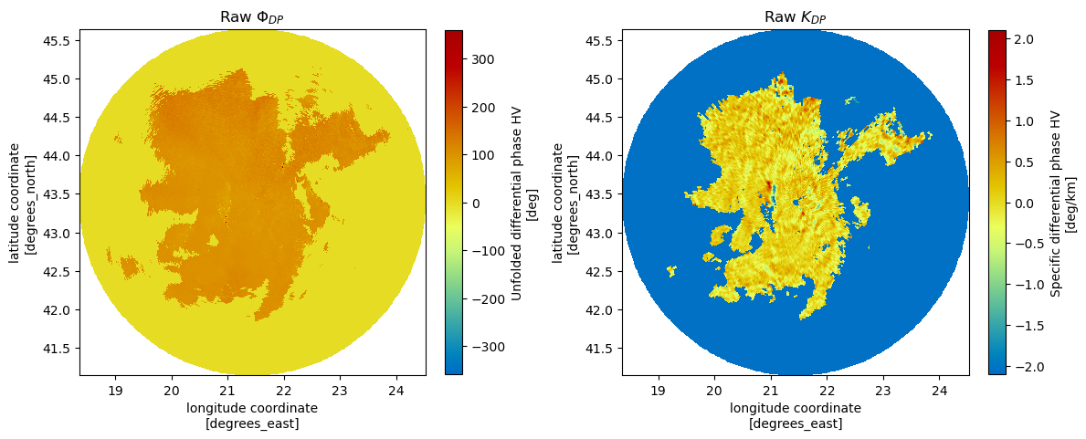

Masked RAW¶

fig, (ax1, ax2) = plt.subplots(1, 2, figsize=(12, 5))
mswp.uPhiDP.isel(vcp_time=vcp).wrl.vis.plot(ax=ax1, vmin=0)
ax1.set_title("Raw $\Phi_{DP}$")
mswp.KDP.isel(vcp_time=vcp).wrl.vis.plot(ax=ax2, vmin=0, vmax=2)
ax2.set_title("Raw $K_{DP}$")
fig.tight_layout()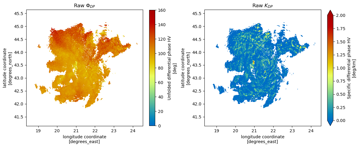

Pre-Processed¶

fig, (ax1, ax2) = plt.subplots(1, 2, figsize=(12, 5))
swp.PHIDP.isel(vcp_time=vcp).wrl.vis.plot(ax=ax1, vmin=0)
ax1.set_title("Pre-processed $\Phi_{DP}$")
mswp.PHIDP.isel(vcp_time=vcp).wrl.vis.plot(ax=ax2, vmin=0)
ax2.set_title("Masked Pre-processed $\Phi_{DP}$")
fig.tight_layout()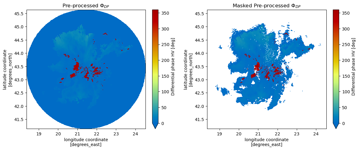

Single Radial¶

fig, (ax1, ax2) = plt.subplots(2, 1, figsize=(12, 10))
az = 280
az_slice = slice(az, az + 1)

sswp = swp.isel(vcp_time=vcp).sel(azimuth=az_slice)
smswp = mswp.isel(vcp_time=vcp).sel(azimuth=az_slice)

(sswp.uPhiDP - system_offset).plot.line(ax=ax1, hue="azimuth", label="phi_raw")
(smswp.uPhiDP - system_offset).plot.line(ax=ax1, hue="azimuth", label="phi_raw_masked")
sswp.PHIDP.plot.line(ax=ax1, hue="azimuth", label="phi_pre")
smswp.PHIDP.plot.line(ax=ax1, hue="azimuth", label="phi_pre_masked")
ax1.set_title("$\Phi_{DP}$")
#ax1.set_ylim(-10, 20)
ax1.legend(loc="upper right")

(sswp.uPhiDP - system_offset).plot.line(ax=ax2, hue="azimuth", label="phi_raw")
sswp.PHIDP.plot.line(ax=ax2, hue="azimuth", label="phi_pre")
ax2.set_title("$\Phi_{DP}$")
ax2.set_ylim(-20, 30)
ax2.legend(loc="upper right")
fig.tight_layout()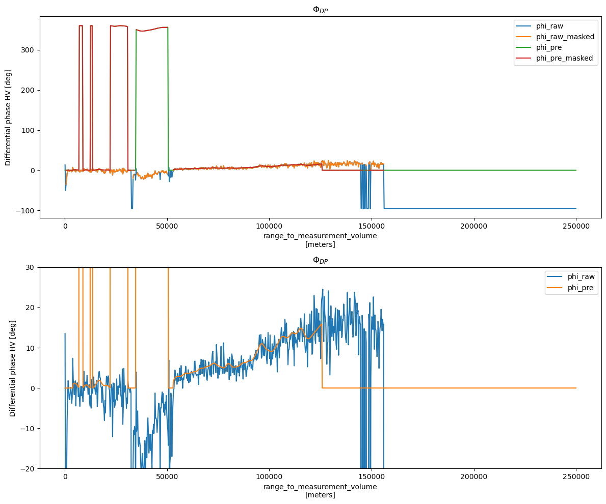

Unfold Phase¶

If your radar suffers from phase folding, eg. the phase wraps at 180° or 360°, depending on layout and continues to increase from -180° or 0° onwards, you would need to properly unfold the phase before any subsequent processing. A common approach is described in Vulpiani et al. (2012). In our case, phase unfolding isn’t an issue, so we skip it.

Derive $K_{DP}$ from $\Phi_{DP}$ ¶

Pre-process PHIDP¶

wradlib implements an optimized wradlib.util.UtilMethods.derivate algorithm which can be shaped for polar phase measurements in wradlib.dp.DpMethods.kdp_from_phidp.

Using the defaults the derivation algorithm uses low-noise Lanczos Differentiators (Diekema & Koornwinder (2012)).

Savitzky-Golay Filter¶

The Savitzky–Golay filter smooths the differential phase by fitting a polynomial within a moving window along each radar ray. Unlike a simple moving average, it reduces measurement noise while preserving the local structure of the phase profile.

A quality mask is then created by retaining only gates whose smoothed differential phase exceeds the system phase offset minus a small tolerance. Gates failing this criterion are excluded from subsequent processing.

Finally despeckling is done.

from scipy.signal import savgol_filter
import xarray as xr

u = mswp.uPhiDP

window_mean = (
    u.rolling(range=7, center=True)
    .construct("window")
    .mean("window")
)

u_filled = u.fillna(window_mean).chunk(range=-1)

phidp_smooth = xr.apply_ufunc(
    savgol_filter,
    u_filled,
    kwargs={
        "window_length": 21,
        "polyorder": 2,
        "axis": -1,
        "mode": "nearest",
    },
    input_core_dims=[["range"]],
    output_core_dims=[["range"]],
    dask="parallelized",
    output_dtypes=[mswp.uPhiDP.dtype],
)

# phidp_smooth = phidp_smooth.interpolate_na("range", method="linear", limit=29)

mask2 = phidp_smooth > (system_offset - 1)
phidp_masked = mswp.uPhiDP.where(mask2).wrl.util.despeckle(n=5)

Get Last valid Phidp range¶

We make use of wradlib.dp.delta_phidp to retrieve a last valid phidp range to mask data.

delta = mswp.uPhiDP.where(~np.isnan(phidp_masked)).wrl.dp.delta_phidp(rng=2000)
display(delta)

mswp.uPhiDP.isel(vcp_time=vcp).sel(azimuth=az_slice).plot.line(hue="azimuth", label="phidp_raw", marker="*")
phidp_masked.isel(vcp_time=vcp).sel(azimuth=az_slice).plot.line(hue="azimuth", label="phidp_masked")
plt.grid()
plt.gca().set_xlim(140e3, 160e3)
delta.isel(vcp_time=vcp).sel(azimuth=az_slice).stop_range.values
plt.gca().set_title("Last Valid PHIDP range - single radial")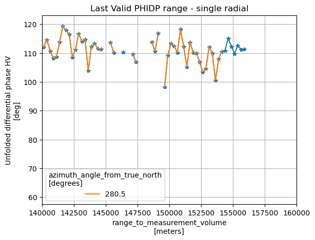

(phidp_masked  - system_offset).isel(vcp_time=vcp).plot(x="azimuth", cmap="HomeyerRainbow", vmin=-10, vmax=60)
delta.isel(vcp_time=vcp).stop_range.plot(color="k")
plt.gca().set_title("Last Valid PHIDP range")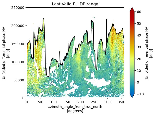

Retrieve smoothed phidp¶

We restrict the raw data by the valid data of our filtered data and our retrival of max PHIDP range.

Finally we linearly interpolate nan along the range on a rolling mean. Attention, this might introduce artifacts.

phidp_mean = mswp.uPhiDP.where(~np.isnan(phidp_masked)).where(mswp.range <= delta.stop_range)
phidp_mean = phidp_mean.interpolate_na("range", method="linear").rolling(
     range=29,
     center=True,
     min_periods=7,
).mean(skipna=True)

fig, (ax1, ax2) = plt.subplots(1, 2, figsize=(12, 5))
(mswp.uPhiDP - system_offset).isel(vcp_time=vcp).wrl.vis.plot(ax=ax1, vmin=0, vmax=60)
ax1.set_title("$\Phi_{DP}$ raw - offset corrected")
(phidp_mean - system_offset).isel(vcp_time=vcp).wrl.vis.plot(ax=ax2, vmin=0, vmax=60)
ax2.set_title("$\Phi_{DP}$ mean - offset corrected")
fig.tight_layout()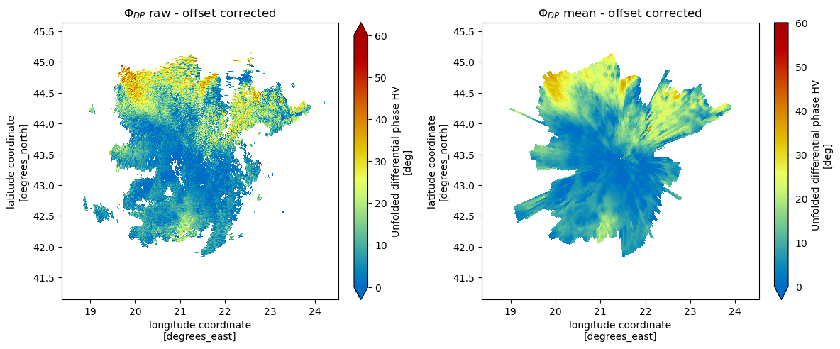

Simple derivation¶

kdp_simple = phidp_mean.wrl.dp.kdp_from_phidp(winlen=27)

Vulpiani algorithm¶

Again in Vulpiani et al. (2012) a full algorithm for derivation of $K_{DP}$ from raw $\Phi_{DP}$ as well as a reprocessed $\Phi_{DP}$ is described (wradlib.dp.DpMethods.phidp_kdp_vulpiani).

phidp_vulpiani, kdp_vulpiani = phidp_mean.copy().wrl.dp.phidp_kdp_vulpiani(winlen=29, niter=5)

Result Plots¶

fig, (ax1, ax2) = plt.subplots(1, 2, figsize=(12, 5))
kdp_simple.isel(vcp_time=vcp).wrl.vis.plot(ax=ax1, vmin=0, vmax=3)
ax1.set_title("$K_{DP}$ simple")
kdp_vulpiani.isel(vcp_time=vcp).wrl.vis.plot(ax=ax2, vmin=0, vmax=3)
ax2.set_title("$K_{DP}$ vulpiani")
fig.tight_layout()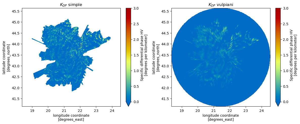

Comparison¶

Let’s have a look at the different evolutions of $\Phi_{DP}$ and $K_{DP}$ .

Single Radial¶

fig, (ax1, ax2) = plt.subplots(2, 1, figsize=(12, 10))
# az = 270
# az = slice(az, az + 1)
(mswp.uPhiDP-system_offset).isel(vcp_time=vcp).sel(azimuth=az_slice).plot.line(ax=ax1, hue="azimuth", label="phidp_raw")
(phidp_smooth-system_offset).isel(vcp_time=vcp).sel(azimuth=az_slice).plot.line(ax=ax1, hue="azimuth", label="phidp_smooth")
(phidp_mean-system_offset).isel(vcp_time=vcp).sel(azimuth=az_slice).ffill("range").plot.line(ax=ax1, hue="azimuth", label="phidp_mean")
(mswp.PHIDP).isel(vcp_time=vcp).sel(azimuth=az_slice).plot.line(ax=ax1, hue="azimuth", label="phidp_corr_sys")
phidp_vulpiani.isel(vcp_time=vcp).sel(azimuth=az_slice).plot.line(ax=ax1, hue="azimuth", label="phidp_vulpiani")
ax1.set_title("$\Phi_{DP}$")
ax1.set_ylim(-10, 30)
ax1.legend(loc="lower right")

mswp.KDP.isel(vcp_time=vcp).sel(azimuth=az_slice).plot.line(ax=ax2, hue="azimuth", label="kdp_raw")
kdp_simple.isel(vcp_time=vcp).sel(azimuth=az_slice).plot.line(ax=ax2, hue="azimuth", label="kdp_simple")
kdp_vulpiani.isel(vcp_time=vcp).sel(azimuth=az_slice).plot.line(ax=ax2, hue="azimuth", label="kdp_vulpiani")
ax2.set_title("$K_{DP}$")
ax2.legend(loc="upper left")
fig.tight_layout()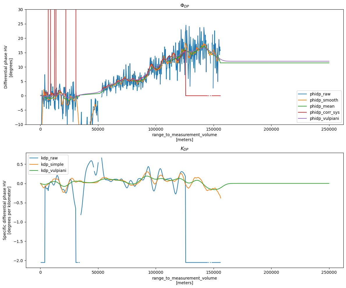

Single Sweep¶

fig, (ax1, ax2, ax3) = plt.subplots(1, 3, figsize=(18, 5))
(mswp.uPhiDP-system_offset).isel(vcp_time=vcp).wrl.vis.plot(ax=ax1, vmin=-10, vmax=60)
ax1.set_title("$\Phi_{DP}$ raw")
(mswp.PHIDP).isel(vcp_time=vcp).wrl.vis.plot(ax=ax2, vmin=-10, vmax=60)
ax2.set_title("$\Phi_{DP}$ corr sys")
(phidp_smooth-system_offset).isel(vcp_time=vcp).wrl.vis.plot(ax=ax3, vmin=-10, vmax=60)
ax3.set_title("$\Phi_{DP}$ smooth")
fig.tight_layout()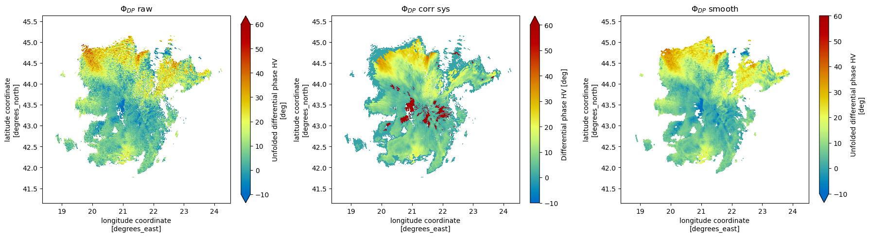

fig, (ax1, ax2) = plt.subplots(1, 2, figsize=(12, 5))
(phidp_mean-system_offset).isel(vcp_time=vcp).wrl.vis.plot(ax=ax1, vmin=0, vmax=60)
ax1.set_title("$\Phi_{DP}$ mean")
phidp_vulpiani.where(~np.isnan(mswp.uPhiDP)).isel(vcp_time=vcp).wrl.vis.plot(ax=ax2, vmin=0, vmax=60)
ax2.set_title("$\Phi_{DP}$ vulpiani")
fig.tight_layout()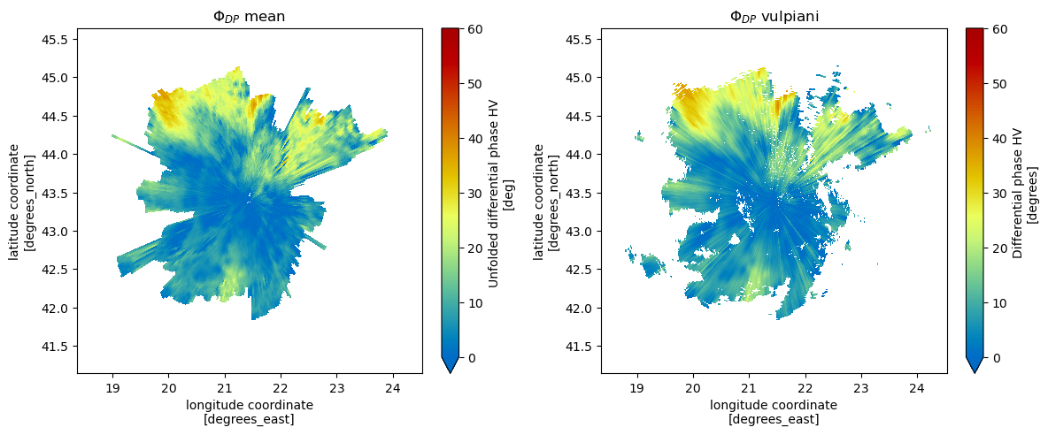

fig, (ax1, ax2, ax3) = plt.subplots(1, 3, figsize=(18, 5))
mswp.KDP.isel(vcp_time=vcp).wrl.vis.plot(ax=ax1, vmin=0, vmax=3)
ax1.set_title("$K_{DP}$ raw")
kdp_simple.isel(vcp_time=vcp).wrl.vis.plot(ax=ax2, vmin=0, vmax=3)
ax2.set_title("$K_{DP}$ simple")
kdp_vulpiani.isel(vcp_time=vcp).wrl.vis.plot(ax=ax3, vmin=0, vmax=3)
ax3.set_title("$K_{DP}$ vulpiani")
fig.tight_layout()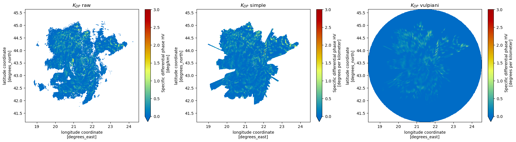

Next Steps¶

You’ve completed the differential phase workflow for the selected dataset. Return to Claim Data, select the other case study day, and rerun the notebook.

References¶

Vulpiani, G., Montopoli, M., Passeri, L. D., Gioia, A. G., Giordano, P., & Marzano, F. S. (2012). On the Use of Dual-Polarized C-Band Radar for Operational Rainfall Retrieval in Mountainous Areas. Journal of Applied Meteorology and Climatology, 51(2), 405–425. 10.1175/jamc-d-10-05024.1
Diekema, E., & Koornwinder, T. H. (2012). Differentiation by integration using orthogonal polynomials, a survey. Journal of Approximation Theory, 164(5), 637–667. 10.1016/j.jat.2012.01.003
Vulpiani, G., Montopoli, M., Passeri, L. D., Gioia, A. G., Giordano, P., & Marzano, F. S. (2012). On the Use of Dual-Polarized C-Band Radar for Operational Rainfall Retrieval in Mountainous Areas. Journal of Applied Meteorology and Climatology, 51(2), 405–425. 10.1175/jamc-d-10-05024.1

Differential Phase

Differential Phase¶

Claim Data¶

Get lowest elevation sweep¶

Mask with RHOHV¶

Overview Plots¶

Select vcp_time index¶

Unmasked RAW¶

Masked RAW¶

Pre-Processed¶

Single Radial¶

Unfold Phase¶

Derive KDPK_{DP}KDP​ from ΦDP\Phi_{DP}ΦDP​¶

Pre-process PHIDP¶

Savitzky-Golay Filter¶

Get Last valid Phidp range¶

Retrieve smoothed phidp¶

Simple derivation¶

Vulpiani algorithm¶

Result Plots¶

Comparison¶

Single Radial¶

Single Sweep¶

Next Steps¶

Derive $K_{DP}$ from $\Phi_{DP}$ ¶