



Total Differential Phase Shift
This notebook focuses on the estimation of the total differential phase shift, , from polarimetric radar observations.
The estimated is an important intermediate quantity in several radar processing tasks, including attenuation correction.
The algorithm is described in detail in Testud et al. (2000), Ryzhkov et al. (2014) and Diederich et al. (2015).
Claim Data
We use the ARCO data provided in Data Access — Serbian Rainbow Radar. Please refer to this notebook for details of access.
OSN_ENDPOINT = "https://umn1.osn.mghpcc.org"
BUCKET = "nexrad-arco"
prefix = "jastrebac_250m" # dual-pol, 12 × 360 × 1000, 2014 only
# prefix = "jastrebac_500m" # dual-pol, 12 × 360 × 500, 2017 + 2026
storage = icechunk.s3_storage(
bucket=BUCKET,
prefix=prefix,
endpoint_url=OSN_ENDPOINT,
region="us-east-1",
anonymous=True,
force_path_style=True,
)
repo = icechunk.Repository.open(storage)
dtree = xr.open_datatree(
repo.readonly_session("main").store,
engine="zarr",
consolidated=False,
chunks={},
)
display(dtree)
root = next(iter(dtree.keys())).split("/")[0]Get lowest elevation sweep
First we get the lowest sweep and do some georeferencing.
swp = (
    dtree[f"{root}/sweep_0"]
    .to_dataset(inherit="all_coords")
    .wrl.georef.georeference(crs=wrl.georef.get_earth_projection())
).sel(vcp_time="2014")
swp.z.attrs = xd.model.get_altitude_attrs()
display(swp)Mask with RHOHV
First, we mask with and/or any other moment you trust to remove unwanted signal.
mask = (swp.RHOHV >= 0.9)
mswp = swp.where(mask)
phimask = mswp.uPhiDP
Estimate 
Second, we estimate total differential phase shift . The range window can be selected according to your data.
dphi = phimask.wrl.dp.delta_phidp(5000.)
display(dphi)Overview Plots
Let’s have a look at the results.
Select vcp_time index
vcp = 0Phase over Azimuth
fig, (ax1, ax2) = plt.subplots(2, 1, figsize=(16, 8))
dphi.first.isel(vcp_time=vcp).plot(label="first", ax=ax1)
dphi.last.isel(vcp_time=vcp).plot(label="last", ax=ax1)
ax1.grid()
ax1.legend()
dphi.dphi.isel(vcp_time=vcp).plot(ls="-", marker=".", label="delta", ax=ax2)
ax2.grid()
ax2.legend()
plt.tight_layout()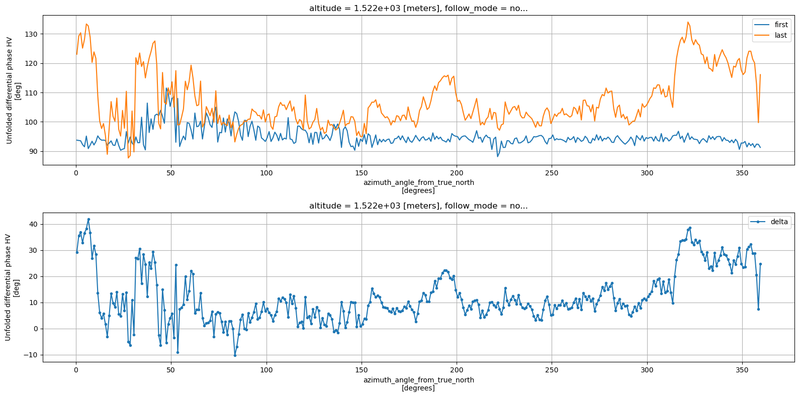
Polar Domain
fig = plt.figure(figsize=(20, 14))
ax1 = plt.subplot(231, projection="polar")
ax2 = plt.subplot(232, projection="polar")
ax3 = plt.subplot(233, projection="polar")
# set the lable go clockwise and start from the top
ax1.set_theta_zero_location("N")
ax2.set_theta_zero_location("N")
ax3.set_theta_zero_location("N")
# clockwise
ax1.set_theta_direction(-1)
ax2.set_theta_direction(-1)
ax3.set_theta_direction(-1)

theta = np.linspace(0, 2 * np.pi, num=360, endpoint=False)
ax1.plot(theta, dphi.first_idx.isel(vcp_time=vcp), color="b", linewidth=3)
_ = ax1.set_title(r"$\Delta \Phi_{DP}$ - First Index")
ax2.plot(theta, dphi.last_idx.isel(vcp_time=vcp), color="r", linewidth=3)
_ = ax2.set_title(r"$\Delta \Phi_{DP}$ - Last Index")
ax3.plot(theta, dphi.dphi.isel(vcp_time=vcp), color="g", linewidth=3)
_ = ax3.set_title(r"$\Delta \Phi_{DP}^{tot}$")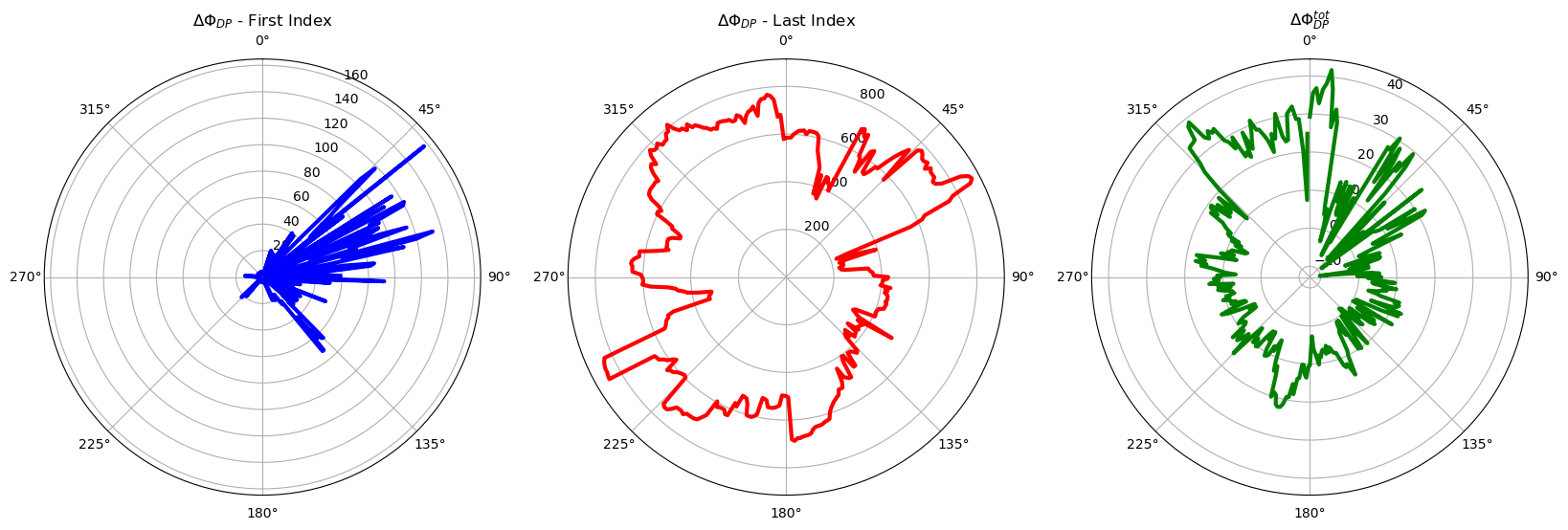
First and last segments
fig, (ax1, ax2) = plt.subplots(2, 1, figsize=(10, 10), sharex=True)
dphi.start_range.isel(vcp_time=vcp).plot(ax=ax1, lw=0.8, c="k")
(dphi.start_range.isel(vcp_time=vcp) + dphi.center_span).plot(ax=ax1, lw=0.8, c="r", ls=":")
dphi.stop_range.isel(vcp_time=vcp).plot(ax=ax1, lw=0.8, c="k")
(dphi.stop_range.isel(vcp_time=vcp) - dphi.center_span).plot(ax=ax1, lw=0.8, c="r", ls=":")
phimask.isel(vcp_time=vcp).plot(ax=ax1, x="azimuth", y="range", cmap="turbo", vmin=90, vmax=300)
ax1.set_title(r"$\Phi_{DP}$ - start/stop")

phimask2 = phimask.where(((phimask.range >= dphi.start_range.isel(vcp_time=vcp)) & (phimask.range <= dphi.start_range.isel(vcp_time=vcp) + dphi.center_span)) |
                         ((phimask.range >= dphi.stop_range.isel(vcp_time=vcp) - dphi.center_span) & (phimask.range <= dphi.stop_range.isel(vcp_time=vcp))))
phimask2.isel(vcp_time=vcp).plot(ax=ax2, x="azimuth", y="range", cmap="turbo", vmin=90, vmax=300)
dphi.start_range.isel(vcp_time=vcp).plot(ax=ax2, lw=0.8, c="k", ls=":")
(dphi.start_range.isel(vcp_time=vcp) + dphi.center_span).plot(ax=ax2, lw=0.8, c="k", ls=":")
dphi.stop_range.isel(vcp_time=vcp).plot(ax=ax2, lw=0.8, c="k", ls=":")
(dphi.stop_range.isel(vcp_time=vcp) - dphi.center_span).plot(ax=ax2, lw=0.8, c="k", ls=":")
ax2.set_title(r"$\Phi_{DP}$ - start/stop - masked")
fig.tight_layout()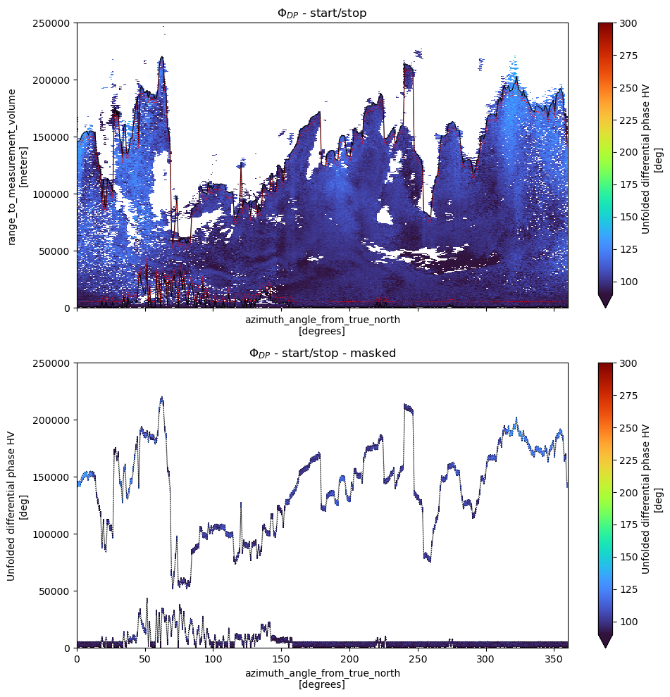
Next Steps
You’ve completed the total differential phase workflow for the selected dataset. Return to Claim Data, select the other case study day, and rerun the notebook.
- Testud, J., Le Bouar, E., Obligis, E., & Ali-Mehenni, M. (2000). The Rain Profiling Algorithm Applied to Polarimetric Weather Radar. Journal of Atmospheric and Oceanic Technology, 17(3), 332–356. https://doi.org/10.1175/1520-0426(2000)017<;0332:trpaat>2.0.co;2
- Ryzhkov, A., Diederich, M., Zhang, P., & Simmer, C. (2014). Potential Utilization of Specific Attenuation for Rainfall Estimation, Mitigation of Partial Beam Blockage, and Radar Networking. Journal of Atmospheric and Oceanic Technology, 31(3), 599–619. 10.1175/jtech-d-13-00038.1
- Diederich, M., Ryzhkov, A., Simmer, C., Zhang, P., & Trömel, S. (2015). Use of Specific Attenuation for Rainfall Measurement at X-Band Radar Wavelengths. Part I: Radar Calibration and Partial Beam Blockage Estimation. Journal of Hydrometeorology, 16(2), 487–502. 10.1175/jhm-d-14-0066.1