Gridding Polar Data¶

import cmweather
import numpy as np
import wradlib as wrl
import matplotlib.pyplot as plt
import xarray as xr
import xradar as xd
import fsspec
import icechunk
import holoviews as hv
import hvplot
import hvplot.xarray
import pyproj
import rioxarray
import warnings
warnings.filterwarnings("ignore", category=RuntimeWarning)
warnings.filterwarnings("ignore", category=FutureWarning)

Claim Data¶

We use the ARCO data provided in Data Access — Serbian Rainbow Radar. Please refer to this notebook for details of access.

OSN_ENDPOINT = "https://umn1.osn.mghpcc.org"
BUCKET = "nexrad-arco"

# prefix = "Fgora"  # single-pol, 12 sweeps × 360 az × 250 range, 2014 + 2017 + 2026
# prefix = "jastrebac_250m"  # dual-pol, 12 × 360 × 1000, 2014 only
prefix = "jastrebac_500m"  # dual-pol, 12 × 360 × 500,  2017 + 2026

storage = icechunk.s3_storage(
    bucket=BUCKET,
    prefix=prefix,
    endpoint_url=OSN_ENDPOINT,
    region="us-east-1",
    anonymous=True,
    force_path_style=True,
)
repo = icechunk.Repository.open(storage)
dtree = xr.open_datatree(
    repo.readonly_session("main").store,
    engine="zarr",
    consolidated=False,
    chunks={},
)
display(dtree)
root = next(iter(dtree.keys())).split("/")[0]

Georeference¶

The Serbian Hydrometeorological Service (RHMZ) radar data used in this workflow is projected in Lambert Azimuthal Equal-Area (LAEA) on the ETRS89 datum, corresponding to EPSG:3035 (ETRS89 / LAEA Europe).

This projection is standard for EUMETNET OPERA radar mosaics and provides a regular, equal-area Cartesian grid (~1 km resolution) suitable for PySTEPS nowcasting, preserving spatial consistency for advection and interpolation.

We’ll use the lowest elevation as an example.

sweep = "sweep_0"

x0 = 3760756.2464729655
y0 = -2656141.3006878751

proj_laea = pyproj.CRS.from_proj4(
    "+proj=laea +lat_0=52 +lon_0=10 "
    f"+x_0={x0} "
    f"+y_0={y0} "
    "+a=6378137 +b=6356752.3141403701 +units=m +no_defs"
)

proj_laea = wrl.georef.ensure_crs(proj_laea)

swp = (
    dtree[f"{root}/{sweep}"]
    .to_dataset()
    .assign_coords(dtree[root].coords)
    .assign_coords(sweep_mode="azimuth_surveillance")
    .wrl.georef.georeference(crs=proj_laea)
)
swp = swp.rename(crs_wkt="spatial_ref")
display(swp)

Create cartesian dataset¶

The x,y-dimension sizes are, as the projection above, taken from the EuCom XL product of The Deutscher Wetterdienst.

nx = 6500
ny = 5300
res = 1000.0

x = x0 + (np.arange(nx) - nx / 2 + 0.5) * res
y = y0 + (np.arange(ny) - ny / 2 + 0.5) * (-res)

cart = xr.Dataset(
    coords={
        "x": ("x", x),
        "y": ("y", y),
    }
).chunk(x=500, y=500)

cart = cart.rio.write_crs(proj_laea)
display(cart)

cart = cart.sel(
    x=slice(swp.x.min(), swp.x.max()),
    y=slice(swp.y.max(), swp.y.min())  # note: y often decreases from north to south
)
display(cart)

Get KDTree mapping¶

First, we build the KDTree mapping swp vs cart.

mapping = swp.wrl.ipol.get_mapping(cart, k=4)
display(mapping)

Run Interpolator¶

The interpolator can now be called with the pre-computed mapping. We take nearest and inverse_distance interpolation schemes. The interpolators can be parameterized via keyword arguments, please refer to the documentation below.

swp_nearest = swp.wrl.ipol.interpolate(mapping, method="nearest")
swp_idw = swp.wrl.ipol.interpolate(mapping, method="inverse_distance", idw_p=2)
display(swp_nearest)
display(swp_idw)

Plot Gridded Data¶

Now, let’s have a look at the created cartesian datasets.

Matplotlib¶

fig = plt.figure(figsize=(12, 10))

kwargs = dict(vmin=0, vmax=60)
kw_lim = dict(xlim=(4.7e6, 4.75e6), ylim=(-3.6e6, -3.65e6))
vcp_dt = swp_nearest.isel(vcp_time=0).vcp_time.values.astype("datetime64[s]")
swp_nearest.DBTH.isel(vcp_time=0).wrl.vis.plot(ax=221, **kwargs)
plt.gca().set_title(f"{vcp_dt}, DBTH - nearest")
swp_idw.DBTH.isel(vcp_time=0).wrl.vis.plot(ax=222, **kwargs)
plt.gca().set_title(f"{vcp_dt}, DBTH - inverse distance")

swp_nearest.DBTH.isel(vcp_time=0).wrl.vis.plot(ax=223, **kwargs, **kw_lim)
plt.gca().set_title(f"{vcp_dt}, DBTH - nearest")
swp_idw.DBTH.isel(vcp_time=0).wrl.vis.plot(ax=224, **kwargs, **kw_lim)
plt.gca().set_title(f"{vcp_dt}, DBTH - inverse distance")
fig.tight_layout()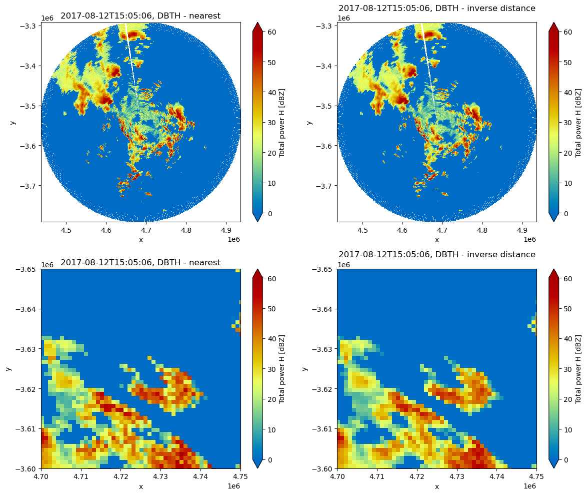

HVPlot¶

hv.extension('bokeh')
hv.output(widget_location="bottom")

swpx = swp_nearest.chunk()
display(swpx)

dbz_opts = dict(
    cmap="HomeyerRainbow", 
    clim=(0, 60), 
    aspect=1
)

vrad_opts = dict(
    cmap="Seismic", 
    clim=(-15, 15), 
    aspect=1
)

wrad_opts = dict(
    cmap="Seismic", 
    clim=(0, 15), 
    aspect=1
)

zdr_opts = dict(
    cmap="HomeyerRainbow", 
    clim=(-0.5, 5), 
    aspect=1
)

rho_opts = dict(
    cmap="plasmidis", 
    clim=(0.0, 1.0), 
    aspect=1
)

phi_opts = dict(
    cmap="Seismic", 
    clim=(0, 60), 
    aspect=1
)

kdp_opts = dict(
    cmap="Seismic", 
    clim=(-0.5, 2), 
    aspect=1
)

moment = swp_nearest["DBTH"].hvplot(x="x", y="y", 
                                   widget_type="scrubber", 
                                   rasterize=True,
                                   widget_location='bottom',
                                   frame_width=500,
                                   **dbz_opts,
                                  )

moment

Write Gridded Data¶

Finally, we write out the data to disk (NetCDF4) for later compositing.

outname_nearest = f"{prefix}_{sweep}_grid_nearest.nc"
swp_nearest.to_netcdf(outname_nearest)

outname_idw = f"{prefix}_{sweep}_grid_idw.nc"
swp_idw.to_netcdf(outname_idw)

swp1 = xr.open_dataset(outname_nearest)
display(swp1)

swp2 = xr.open_dataset(outname_idw)
display(swp2)

Next Steps¶

You’ve completed the gridding workflow for the selected dataset. Return to prefix selection step, choose one of the remaining datasets, and rerun the notebook. Repeat this until all three datasets have been processed.