Inspect Dual Pol Data - Jastrebac¶

Jastrebac radar is located on top of the mountain range of the same name Jastrebac west of Niŝ.

import cmweather
import numpy as np
import wradlib as wrl
import matplotlib.pyplot as plt
import xarray as xr
import xradar as xd
import fsspec
import icechunk
import holoviews as hv
import hvplot
import hvplot.xarray

Claim Data¶

We use the ARCO data provided in Data Access — Serbian Rainbow Radar. Please refer to this notebook for details of access.

OSN_ENDPOINT = "https://umn1.osn.mghpcc.org"
BUCKET = "nexrad-arco"

# prefix = "jastrebac_250m"  # dual-pol, 12 × 360 × 1000, 2014 only
prefix = "jastrebac_500m"  # dual-pol, 12 × 360 × 500,  2017 + 2026

storage = icechunk.s3_storage(
    bucket=BUCKET,
    prefix=prefix,
    endpoint_url=OSN_ENDPOINT,
    region="us-east-1",
    anonymous=True,
    force_path_style=True,
)
repo = icechunk.Repository.open(storage)
dtree = xr.open_datatree(
    repo.readonly_session("main").store,
    engine="zarr",
    consolidated=False,
    chunks={},
)
display(dtree)
root = next(iter(dtree.keys())).split("/")[0]

Radar domain¶

Get lowest elevation sweep¶

First we get the lowest sweep and do some georeferencing.

swp = (
    dtree[f"{root}/sweep_0"]
    .to_dataset()
    .assign_coords(dtree[root].coords)
    .assign_coords(sweep_mode="azimuth_surveillance")
    .wrl.georef.georeference(crs=wrl.georef.get_earth_projection())
)
swp.x.attrs = xd.model.get_longitude_attrs()
swp.y.attrs = xd.model.get_latitude_attrs()
swp.z.attrs = xd.model.get_altitude_attrs()
display(swp)

Plot over Maptiles¶

Use the bokeh infrastructure to interact with the plot.

import holoviews as hv
import geopandas as gpd
from shapely.geometry import Point
import hvplot.pandas

lon, lat = swp.longitude.values, swp.latitude.values

radar = gpd.GeoDataFrame(
    geometry=[
        Point(lon, lat),
    ],
    crs="EPSG:4326",
)

lon_domain = swp.isel(range=-1).x.values
lat_domain = swp.isel(range=-1).y.values
ring = gpd.GeoDataFrame(
    geometry=[Point(xy) for xy in zip(lon_domain, lat_domain)],
    crs="EPSG:4326"
)

tiles = hv.element.tiles.OpenTopoMap()

points = radar.hvplot.points(
    x="lon",
    y="lat",
    marker="o",
    geo=True,
    s=100,
    c="red",
    tiles=tiles,
)

domain = ring.hvplot(
    geo=True,
    line_width=2,
    color="blue",
)

(points * domain).opts(
    frame_width=600,
    # height=600,
)

Scan pattern¶

TTo visualize the scan pattern we just select a single volume.

svol = dtree[root].isel(vcp_time=0)
display(svol)
for c, v in svol.coords.items():
    print(c, v.values)
for c in sorted(svol.children, key=lambda x: int(x.split("_")[-1])):
    print(c, svol[c].time.isel(azimuth=0).values)

altitude 1522.0
latitude 43.39116
prt_mode not_set
follow_mode not_set
longitude 21.44335
vcp_time 2017-08-12T15:05:06.000000000
sweep_mode azimuth_surveillance
sweep_0 2017-08-12T15:05:07.854166528
sweep_1 2017-08-12T15:05:38.604166400
sweep_2 2017-08-12T15:05:53.479166500
sweep_3 2017-08-12T15:06:08.354166528

sweep_4 2017-08-12T15:06:23.062500096
sweep_5 2017-08-12T15:06:38.604166500
sweep_6 2017-08-12T15:06:53.270833500
sweep_7 2017-08-12T15:07:07.645833472
sweep_8 2017-08-12T15:07:38.104166400

sweep_9 2017-08-12T15:07:52.520833500
sweep_10 2017-08-12T15:08:07.687500000
sweep_11 2017-08-12T15:08:22.770833500

ax = svol.wrl.vis.plot_scan_strategy()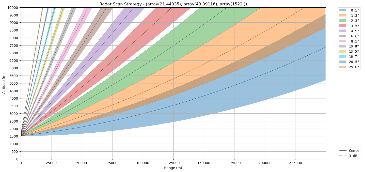

Overview Plot¶

Select a time slot and plot four radar moments!

fig, ((ax1, ax2), (ax3, ax4)) = plt.subplots(2, 2, sharex=True, sharey=True, figsize=(12, 10))
dbz_min, dbz_max = (0, 50)

swp_sel = swp.sel(vcp_time="2014-05-15T00:01:50", method="nearest")

swp_sel.DBTH.wrl.vis.plot(ax=ax1, vmin=dbz_min, vmax=dbz_max)
ax1.set_title("DBTH")
swp_sel.DBZH.wrl.vis.plot(ax=ax2, vmin=dbz_min, vmax=dbz_max)
ax2.set_title("DBZH")
swp_sel.VRADH.wrl.vis.plot(ax=ax3)
ax3.set_title("VRADH")
swp_sel.WRADH.wrl.vis.plot(ax=ax4, vmin=0, vmax=6)
ax4.set_title("WRADH")

fig.tight_layout()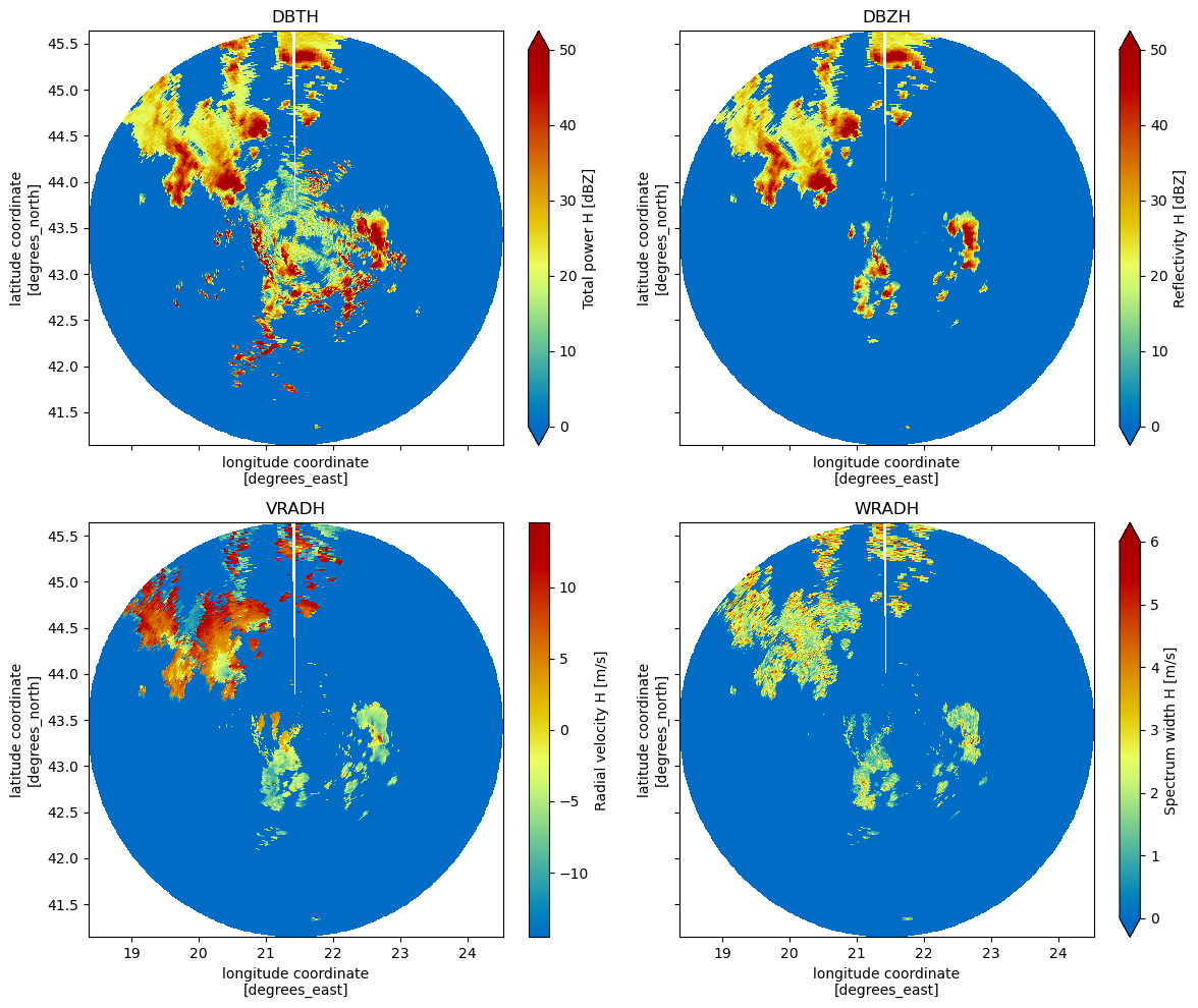

hv.extension('bokeh')
hv.output(widget_location="bottom")

swpx = swp.chunk()

dbz_opts = dict(
    cmap="HomeyerRainbow", 
    clim=(0, 60), 
    aspect=1
)

vrad_opts = dict(
    cmap="Seismic", 
    clim=(-15, 15), 
    aspect=1
)

wrad_opts = dict(
    cmap="Seismic", 
    clim=(0, 15), 
    aspect=1
)


dbth = (
    swpx.hvplot.quadmesh(groupby="vcp_time", x="x", y="y", z="DBTH", frame_width=250, rasterize=True)   
).opts(axiswise=False, xaxis=None, **dbz_opts)

dbzh = (
    swpx.hvplot.quadmesh(groupby="vcp_time", x="x", y="y", z="DBZH", frame_width=250, rasterize=True)   
).opts(axiswise=False, xaxis=None, yaxis=None, **dbz_opts)

vradh = (
    swpx.hvplot.quadmesh(groupby="vcp_time", x="x", y="y", z="VRADH", frame_width=250, rasterize=True)   
).opts(axiswise=False, **vrad_opts)

wradh = (
    swpx.hvplot.quadmesh(groupby="vcp_time", x="x", y="y", z="WRADH", frame_width=250, rasterize=True)   
).opts(axiswise=False, yaxis=None, **vrad_opts)



layout = (dbth + dbzh + vradh + wradh).cols(2)
layout

Overview Polarimetric Data¶

Matplotlib¶

Select a time slot and plot four polarimetric radar moments!

fig, ((ax1, ax2), (ax3, ax4)) = plt.subplots(2, 2, sharex=True, sharey=True, figsize=(12, 10))
dbz_min, dbz_max = (0, 50)

swp_sel = swp.sel(vcp_time="2014-05-15T00:01:50", method="nearest")

swp_sel.ZDR.wrl.vis.plot(ax=ax1, vmin=-0.5, vmax=5)
ax1.set_title("ZDR")
swp_sel.RHOHV.wrl.vis.plot(ax=ax2, cmap="plasmidis")
ax2.set_title("RHOHV")
swp_sel.PHIDP.wrl.vis.plot(ax=ax3, vmin=0, vmax=60, cmap="ChaseSpectral")
ax3.set_title("PHIDP")
swp_sel.KDP.wrl.vis.plot(ax=ax4, vmin=-0.5, vmax=2)
ax4.set_title("KDP")
#
fig.tight_layout()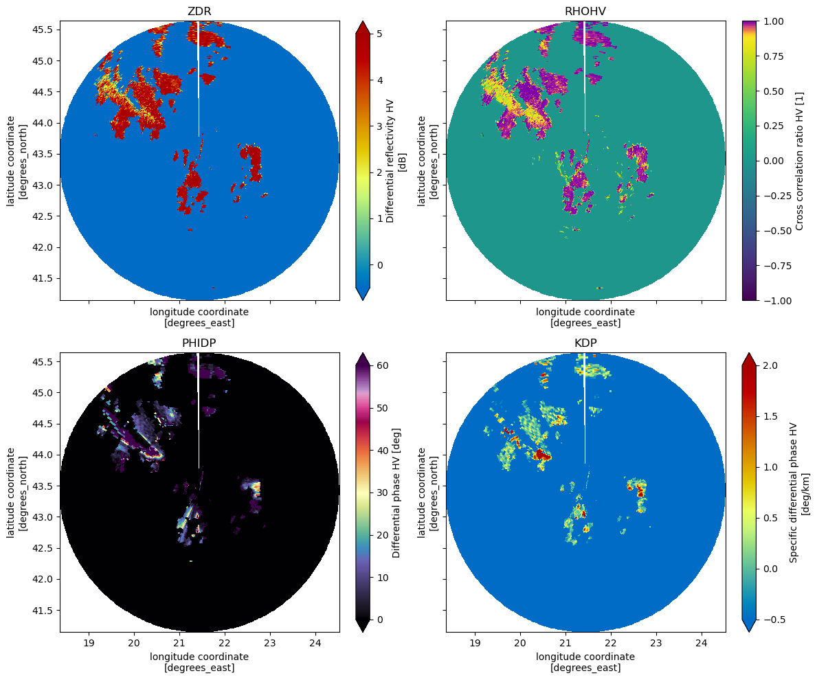

Bokeh¶

hv.extension('bokeh')
hv.output(widget_location="bottom")

swpx = swp.chunk()

zdr_opts = dict(
    cmap="HomeyerRainbow", 
    clim=(-0.5, 5), 
    aspect=1
)

rho_opts = dict(
    cmap="plasmidis", 
    clim=(0.0, 1.0), 
    aspect=1
)

phi_opts = dict(
    cmap="Seismic", 
    clim=(0, 60), 
    aspect=1
)

kdp_opts = dict(
    cmap="Seismic", 
    clim=(-0.5, 2), 
    aspect=1
)

zdr = (
    swpx.hvplot.quadmesh(groupby="vcp_time", x="x", y="y", z="ZDR", frame_width=250, rasterize=True)   
).opts(axiswise=False, xaxis=None, **zdr_opts)

rhohv = (
    swpx.hvplot.quadmesh(groupby="vcp_time", x="x", y="y", z="RHOHV", frame_width=250, rasterize=True)   
).opts(axiswise=False, xaxis=None, yaxis=None, **rho_opts)

phidp = (
    swpx.hvplot.quadmesh(groupby="vcp_time", x="x", y="y", z="PHIDP", frame_width=250, rasterize=True)   
).opts(axiswise=False, **phi_opts)

kdp = (
    swpx.hvplot.quadmesh(groupby="vcp_time", x="x", y="y", z="KDP", frame_width=250, rasterize=True)   
).opts(axiswise=False, yaxis=None, **kdp_opts)

layout = (zdr + rhohv + phidp + kdp).cols(2)
layout