
MetPy for analysis and visualization of diverse data
Overview
MetPy is a collection of tools for reading, managing, analyzing, and visualizing weather data in Python. MetPy is built within and upon the open scientific Python ecosystem, utilizing popular tools like Pandas, Xarray, Cartopy, Pyproj, and more!
Today, we will dive straight in with a crash course on MetPy for the basics of units, data management, and plotting with MetPy. We will end the day with a final plot summarizing multiple data types and calculations alongside previously generated wind retrievals from PyDDA.

Outline
Crash Course to MetPy
Units and
metpy.calcmetpy.iofor reading dataPlotting SkewT’s and Station Plots
xarray + MetPy and CF Conventions
Final Analysis
Imports
import cartopy.crs as ccrs
import matplotlib.pyplot as plt
import numpy as np
import pandas as pd
import pyart.io
import xarray as xr
## You are using the Python ARM Radar Toolkit (Py-ART), an open source
## library for working with weather radar data. Py-ART is partly
## supported by the U.S. Department of Energy as part of the Atmospheric
## Radiation Measurement (ARM) Climate Research Facility, an Office of
## Science user facility.
##
## If you use this software to prepare a publication, please cite:
##
##     JJ Helmus and SM Collis, JORS 2016, doi: 10.5334/jors.119
Crash Course to MetPy
Units and calculations
MetPy requires units for correctness and unit-aware analysis across the package through the use of Pint. We can get started with an import and defining our first Quantity.
from metpy.units import units
miles = units.Quantity(3.5, "miles")
hour = 0.5 * units.hr
# Those are the same!

print(miles, hour)
3.5 mile 0.5 hour
speed = miles / hour
speed
Pint gives us a variety of helpful methods for converting and reducing units.
speed.to("m/s")
Temperature is a common one! Watch out for degC vs. C.
temp_outside = 25 * units.degC
temp_increase = 2.5 * units.degC

temp_outside + temp_increase
---------------------------------------------------------------------------
OffsetUnitCalculusError                   Traceback (most recent call last)
Cell In[6], line 4
      1 temp_outside = 25 * units.degC
      2 temp_increase = 2.5 * units.degC
----> 4 temp_outside + temp_increase

File ~/mambaforge/envs/ams-open-radar-2023-dev/lib/python3.11/site-packages/pint/facets/plain/quantity.py:829, in PlainQuantity.__add__(self, other)
    826 if isinstance(other, datetime.datetime):
    827     return self.to_timedelta() + other
--> 829 return self._add_sub(other, operator.add)

File ~/mambaforge/envs/ams-open-radar-2023-dev/lib/python3.11/site-packages/pint/facets/plain/quantity.py:100, in check_implemented.<locals>.wrapped(self, *args, **kwargs)
     98 elif isinstance(other, list) and other and isinstance(other[0], type(self)):
     99     return NotImplemented
--> 100 return f(self, *args, **kwargs)

File ~/mambaforge/envs/ams-open-radar-2023-dev/lib/python3.11/site-packages/pint/facets/plain/quantity.py:805, in PlainQuantity._add_sub(self, other, op)
    803     units = other._units
    804 else:
--> 805     raise OffsetUnitCalculusError(self._units, other._units)
    807 return self.__class__(magnitude, units)

OffsetUnitCalculusError: Ambiguous operation with offset unit (degree_Celsius, degree_Celsius). See https://pint.readthedocs.io/en/stable/user/nonmult.html for guidance.
What the heck happened there?
temp_inside = 21 * units.degC

temp_outside - temp_inside
temp_increase = 2.5 * units.delta_degC

temp_outside + temp_increase
This can save you from weird errors and science headaches, and all of MetPy’s calculations require units and process the information for you throughout your workflows.
import metpy.calc as mpcalc
u = 30 * units.knots
v = 5 * units.kg

mpcalc.wind_direction(u, v)
---------------------------------------------------------------------------
ValueError                                Traceback (most recent call last)
Cell In[10], line 4
      1 u = 30 * units.knots
      2 v = 5 * units.kg
----> 4 mpcalc.wind_direction(u, v)

File ~/mambaforge/envs/ams-open-radar-2023-dev/lib/python3.11/site-packages/metpy/xarray.py:1328, in preprocess_and_wrap.<locals>.decorator.<locals>.wrapper(*args, **kwargs)
   1325     _mutate_arguments(bound_args, units.Quantity, lambda arg, _: arg.m)
   1327 # Evaluate inner calculation
-> 1328 result = func(*bound_args.args, **bound_args.kwargs)
   1330 # Wrap output based on match and match_unit
   1331 if match is None:

File ~/mambaforge/envs/ams-open-radar-2023-dev/lib/python3.11/site-packages/metpy/units.py:324, in check_units.<locals>.dec.<locals>.wrapper(*args, **kwargs)
    322 @functools.wraps(func)
    323 def wrapper(*args, **kwargs):
--> 324     _check_units_inner_helper(func, sig, defaults, dims, *args, **kwargs)
    325     return func(*args, **kwargs)

File ~/mambaforge/envs/ams-open-radar-2023-dev/lib/python3.11/site-packages/metpy/units.py:311, in _check_units_inner_helper(func, sig, defaults, dims, *args, **kwargs)
    306         if changed_version:
    307             msg = (
    308                 f'This function changed in {changed_version}--double check '
    309                 'that the function is being called properly.\n'
    310             ) + msg
--> 311     raise ValueError(msg)
    313 # Return the bound arguments for reuse
    314 return bound_args

ValueError: `wind_direction` given arguments with incorrect units: `v` requires "[speed]" but given "kilogram"
u = 10 * units.kts
v = 5 * units("m/s")

mpcalc.wind_direction(u, v)
MetPy for annoying data you love
The title says it all.

Let’s start with a classic, METARs.
from metpy.io import parse_metar_file
df = pd.read_csv("../../data/metpy/asos.csv")
df.head()
| KMDQ 110000Z AUTO 16013G19KT 10SM SCT047 OVC050 25/15 A2985 RMK AO2 LTG DSNT NW | |
|---|---|
| 0 | KMDQ 110020Z AUTO 17009G17KT 10SM SCT048 BKN06... |
| 1 | KMDQ 110040Z AUTO 16010G16KT 10SM BKN044 BKN05... |
| 2 | METAR KHSV 110053Z 17014KT 10SM BKN040 BKN055 ... |
| 3 | KDCU 110053Z AUTO 17013G20KT 10SM FEW060 23/17... |
| 4 | KMDQ 110100Z AUTO 17010G17KT 10SM SCT044 SCT04... |
Now, that’s not particularly helpful. But I know there’s some meaningful information in those reports. Let’s parse it.
metars = parse_metar_file("../../data/metpy/asos.csv", month=4, year=2008).set_index("date_time")
metars
Downloading file 'sfstns.tbl' from 'https://github.com/Unidata/MetPy/raw/v1.5.1/staticdata/sfstns.tbl' to '/home/dcamron/.cache/metpy/v1.5.1'.
Downloading file 'master.txt' from 'https://github.com/Unidata/MetPy/raw/v1.5.1/staticdata/master.txt' to '/home/dcamron/.cache/metpy/v1.5.1'.
Downloading file 'stations.txt' from 'https://github.com/Unidata/MetPy/raw/v1.5.1/staticdata/stations.txt' to '/home/dcamron/.cache/metpy/v1.5.1'.
Downloading file 'airport-codes.csv' from 'https://github.com/Unidata/MetPy/raw/v1.5.1/staticdata/airport-codes.csv' to '/home/dcamron/.cache/metpy/v1.5.1'.
| station_id | latitude | longitude | elevation | wind_direction | wind_speed | wind_gust | visibility | current_wx1 | current_wx2 | ... | air_temperature | dew_point_temperature | altimeter | current_wx1_symbol | current_wx2_symbol | current_wx3_symbol | remarks | air_pressure_at_sea_level | eastward_wind | northward_wind | |
|---|---|---|---|---|---|---|---|---|---|---|---|---|---|---|---|---|---|---|---|---|---|
| date_time | |||||||||||||||||||||
| 2008-04-11 00:00:00 | KMDQ | 34.86 | -86.55 | 230 | 160 | 13.0 | 19.0 | 16093.44 | NaN | NaN | ... | 25.0 | 15.0 | 29.85 | 0 | 0 | 0 | AO2 LTG DSNT NW | 1010.12 | -4.446262e+00 | 12.216004 |
| 2008-04-11 00:20:00 | KMDQ | 34.86 | -86.55 | 230 | 170 | 9.0 | 17.0 | 16093.44 | NaN | NaN | ... | 25.0 | 15.0 | 29.85 | 0 | 0 | 0 | AO2 | 1010.12 | -1.562834e+00 | 8.863270 |
| 2008-04-11 00:40:00 | KMDQ | 34.86 | -86.55 | 230 | 160 | 10.0 | 16.0 | 16093.44 | NaN | NaN | ... | 25.0 | 15.0 | 29.85 | 0 | 0 | 0 | AO2 | 1010.12 | -3.420201e+00 | 9.396926 |
| 2008-04-11 00:53:00 | KHSV | 34.65 | -86.78 | 191 | 170 | 14.0 | NaN | 16093.44 | NaN | NaN | ... | 24.0 | 17.0 | 29.86 | 0 | 0 | 0 | AO2 SLP106 T02440167 | 1010.72 | -2.431074e+00 | 13.787309 |
| 2008-04-11 00:53:00 | KDCU | 34.65 | -86.95 | 176 | 170 | 13.0 | 20.0 | 16093.44 | NaN | NaN | ... | 23.0 | 17.0 | 29.84 | 0 | 0 | 0 | AO2 SLP100 T02330172 | 1010.17 | -2.257426e+00 | 12.802501 |
| ... | ... | ... | ... | ... | ... | ... | ... | ... | ... | ... | ... | ... | ... | ... | ... | ... | ... | ... | ... | ... | ... |
| 2008-04-11 22:53:00 | KHSV | 34.65 | -86.78 | 191 | 230 | 9.0 | NaN | 16093.44 | NaN | NaN | ... | 21.0 | 12.0 | 29.79 | 0 | 0 | 0 | AO2 SLP082 T02110122 | 1008.57 | 6.894400e+00 | 5.785088 |
| 2008-04-11 23:00:00 | KMDQ | 34.86 | -86.55 | 230 | 200 | 8.0 | NaN | 16093.44 | NaN | NaN | ... | 21.0 | 16.0 | 29.78 | 0 | 0 | 0 | AO2 | 1008.10 | 2.736161e+00 | 7.517541 |
| 2008-04-11 23:20:00 | KMDQ | 34.86 | -86.55 | 230 | 190 | 7.0 | NaN | 16093.44 | NaN | NaN | ... | 20.0 | 13.0 | 29.77 | 0 | 0 | 0 | AO2 LTG DSNT E AND S | 1007.85 | 1.215537e+00 | 6.893654 |
| 2008-04-11 23:40:00 | KMDQ | 34.86 | -86.55 | 230 | 180 | 6.0 | NaN | 16093.44 | NaN | NaN | ... | 20.0 | 15.0 | 29.77 | 0 | 0 | 0 | AO2 LTG DSNT E | 1007.85 | -7.347881e-16 | 6.000000 |
| 2008-04-11 23:53:00 | KHSV | 34.65 | -86.78 | 191 | 190 | 4.0 | NaN | 16093.44 | NaN | NaN | ... | 21.0 | 16.0 | 29.79 | 0 | 0 | 0 | AO2 SLP082 8/07/ BINOVC 60085 T02060156 10272 ... | 1008.57 | 6.945927e-01 | 3.939231 |
155 rows × 30 columns
Much better! Now we can use pandas for all of the subsetting and exploration we’re used to.
subset = metars.loc["2008-04-11 18:25:00": "2008-04-11 18:40:00"]
subset
| station_id | latitude | longitude | elevation | wind_direction | wind_speed | wind_gust | visibility | current_wx1 | current_wx2 | ... | air_temperature | dew_point_temperature | altimeter | current_wx1_symbol | current_wx2_symbol | current_wx3_symbol | remarks | air_pressure_at_sea_level | eastward_wind | northward_wind | |
|---|---|---|---|---|---|---|---|---|---|---|---|---|---|---|---|---|---|---|---|---|---|
| date_time | |||||||||||||||||||||
| 2008-04-11 18:30:00 | KDCU | 34.65 | -86.95 | 176 | 220 | 10.0 | 28.0 | 11265.408 | -TSRA | NaN | ... | 23.0 | 19.0 | 29.75 | 1095 | 0 | 0 | AO2 PK WND 20030/1820 LTG DSNT ALQDS TSB24RAB0... | 1007.11 | 6.427876 | 7.660444 |
| 2008-04-11 18:40:00 | KMDQ | 34.86 | -86.55 | 230 | 190 | 21.0 | 26.0 | 11265.408 | -VCTSRA | NaN | ... | 24.0 | 18.0 | 29.74 | 1095 | 0 | 0 | AO2 LTG DSNT ALQS | 1006.47 | 3.646612 | 20.680963 |
2 rows × 30 columns
And we can discover a wealth of parsed information available to us for analysis and plotting later.
subset.columns
Index(['station_id', 'latitude', 'longitude', 'elevation', 'wind_direction',
       'wind_speed', 'wind_gust', 'visibility', 'current_wx1', 'current_wx2',
       'current_wx3', 'low_cloud_type', 'low_cloud_level', 'medium_cloud_type',
       'medium_cloud_level', 'high_cloud_type', 'high_cloud_level',
       'highest_cloud_type', 'highest_cloud_level', 'cloud_coverage',
       'air_temperature', 'dew_point_temperature', 'altimeter',
       'current_wx1_symbol', 'current_wx2_symbol', 'current_wx3_symbol',
       'remarks', 'air_pressure_at_sea_level', 'eastward_wind',
       'northward_wind'],
      dtype='object')
MetPy for plots you love
Speaking of, we’ll leave our METARs behind for now, but let’s explore what making plots can look like with MetPy. First, a fan favorite: Skew T diagrams! Let’s explore the 12Z sounding out of Birmingham on the day of our case study.
df = pd.read_fwf("../../data/sounding_data/bmx_sounding_20080411_12Z.txt")
df
| ----------------------------------------------------------------------------- | |
|---|---|
| 0 | PRES HGHT TEMP DWPT RELH MIXR DRCT... |
| 1 | hPa m C C % g/kg deg ... |
| 2 | ----------------------------------------------... |
| 3 | 1000.0 110 |
| 4 | 993.0 178 19.0 17.0 88 12.42 16... |
| ... | ... |
| 136 | 10.5 30480 -47.4 -82.4 1 0.04 310... |
| 137 | 10.0 30780 -47.5 -82.5 1 0.04 280... |
| 138 | 8.7 31716 -39.5 -76.5 1 0.13 ... |
| 139 | 8.7 31699 -39.6 -76.6 1 0.13 275 ... |
| 140 | 8.4 31956 -39.1 -76.1 1 0.15 ... |
141 rows × 1 columns
One more, not particularly helpful. With some exploration and copying and pasting from the file, we can clean up our dataframe a bit.
names_header = "   PRES   HGHT   TEMP   DWPT   RELH   MIXR   DRCT   SKNT   THTA   THTE   THTV"

# slight tweak
units_header = "    hPa     m      degC      degC      %    g/kg    deg   knot     K      K      K "

df = pd.read_fwf("../../data/sounding_data/bmx_sounding_20080411_12Z.txt",
                header=None, skiprows=4, names=names_header.split())
df
| PRES | HGHT | TEMP | DWPT | RELH | MIXR | DRCT | SKNT | THTA | THTE | THTV | |
|---|---|---|---|---|---|---|---|---|---|---|---|
| 0 | 1000.0 | 110 | NaN | NaN | NaN | NaN | NaN | NaN | NaN | NaN | NaN |
| 1 | 993.0 | 178 | 19.0 | 17.0 | 88.0 | 12.42 | 160.0 | 9.0 | 292.7 | 328.2 | 294.9 |
| 2 | 988.0 | 221 | 18.8 | 16.6 | 87.0 | 12.17 | 164.0 | 11.0 | 293.0 | 327.8 | 295.1 |
| 3 | 959.0 | 474 | 17.0 | 16.6 | 97.0 | 12.54 | 187.0 | 23.0 | 293.6 | 329.6 | 295.9 |
| 4 | 943.7 | 610 | 17.1 | 16.8 | 98.0 | 12.94 | 200.0 | 29.0 | 295.1 | 332.4 | 297.4 |
| ... | ... | ... | ... | ... | ... | ... | ... | ... | ... | ... | ... |
| 133 | 10.5 | 30480 | -47.4 | -82.4 | 1.0 | 0.04 | 310.0 | 12.0 | 830.5 | 831.1 | 830.6 |
| 134 | 10.0 | 30780 | -47.5 | -82.5 | 1.0 | 0.04 | 280.0 | 7.0 | 841.1 | 841.7 | 841.1 |
| 135 | 8.7 | 31716 | -39.5 | -76.5 | 1.0 | 0.13 | NaN | NaN | 906.3 | 908.1 | 906.4 |
| 136 | 8.7 | 31699 | -39.6 | -76.6 | 1.0 | 0.13 | 275.0 | 14.0 | 905.1 | 906.8 | 905.1 |
| 137 | 8.4 | 31956 | -39.1 | -76.1 | 1.0 | 0.15 | NaN | NaN | 917.0 | 919.0 | 917.1 |
138 rows × 11 columns
That’s a good start. Let’s get rid of a bunch of our missing data,
df = df.dropna(subset=('TEMP', 'DWPT', 'DRCT', 'SKNT'), how="all").reset_index(drop=True)
df
| PRES | HGHT | TEMP | DWPT | RELH | MIXR | DRCT | SKNT | THTA | THTE | THTV | |
|---|---|---|---|---|---|---|---|---|---|---|---|
| 0 | 993.0 | 178 | 19.0 | 17.0 | 88.0 | 12.42 | 160.0 | 9.0 | 292.7 | 328.2 | 294.9 |
| 1 | 988.0 | 221 | 18.8 | 16.6 | 87.0 | 12.17 | 164.0 | 11.0 | 293.0 | 327.8 | 295.1 |
| 2 | 959.0 | 474 | 17.0 | 16.6 | 97.0 | 12.54 | 187.0 | 23.0 | 293.6 | 329.6 | 295.9 |
| 3 | 943.7 | 610 | 17.1 | 16.8 | 98.0 | 12.94 | 200.0 | 29.0 | 295.1 | 332.4 | 297.4 |
| 4 | 926.0 | 770 | 17.2 | 17.1 | 99.0 | 13.43 | 205.0 | 35.0 | 296.8 | 335.8 | 299.2 |
| ... | ... | ... | ... | ... | ... | ... | ... | ... | ... | ... | ... |
| 132 | 10.5 | 30480 | -47.4 | -82.4 | 1.0 | 0.04 | 310.0 | 12.0 | 830.5 | 831.1 | 830.6 |
| 133 | 10.0 | 30780 | -47.5 | -82.5 | 1.0 | 0.04 | 280.0 | 7.0 | 841.1 | 841.7 | 841.1 |
| 134 | 8.7 | 31716 | -39.5 | -76.5 | 1.0 | 0.13 | NaN | NaN | 906.3 | 908.1 | 906.4 |
| 135 | 8.7 | 31699 | -39.6 | -76.6 | 1.0 | 0.13 | 275.0 | 14.0 | 905.1 | 906.8 | 905.1 |
| 136 | 8.4 | 31956 | -39.1 | -76.1 | 1.0 | 0.15 | NaN | NaN | 917.0 | 919.0 | 917.1 |
137 rows × 11 columns
Now, a tool you might not require often, but can save you some time when you do. Combining pandas with units! Let’s start by constructing a dict of our unit strings that matches each of the columns of df.
from metpy.units import pandas_dataframe_to_unit_arrays

units_dict = {col: unit for col, unit in zip(names_header.split(), units_header.split())}
units_dict
{'PRES': 'hPa',
 'HGHT': 'm',
 'TEMP': 'degC',
 'DWPT': 'degC',
 'RELH': '%',
 'MIXR': 'g/kg',
 'DRCT': 'deg',
 'SKNT': 'knot',
 'THTA': 'K',
 'THTE': 'K',
 'THTV': 'K'}
Now with those…
data = pandas_dataframe_to_unit_arrays(df, units_dict)
data["PRES"]
| Magnitude | [993.0 988.0 959.0 943.7 926.0 925.0 916.0 910.5 906.0 878.4 850.0 845.0 |
|---|---|
| Units | hectopascal |
Of course, you can tackle this by hand for each column whenever you need.
df["PRES"].values * units.hPa
| Magnitude | [993.0 988.0 959.0 943.7 926.0 925.0 916.0 910.5 906.0 878.4 850.0 845.0 |
|---|---|
| Units | hectopascal |
But let’s go back to the unit array dictionary we created above, and pull out our Skew T relevant quantities.
p = data["PRES"]
t = data["TEMP"]
td = data["DWPT"]
And sneak in a calculation to convert from wind speed and direction to u- and v-components of our wind vectors.
u, v = mpcalc.wind_components(data["SKNT"], data["DRCT"])
u
| Magnitude | [-3.07818128993102 -3.0320109139869915 2.802994898318388 9.91858415644439 |
|---|---|
| Units | knot |
Units! Alright, let’s dive in to a Skew T.
from metpy.plots import SkewT
fig = plt.figure()

skew = SkewT(fig, rotation=45)

orangeish = "#d95f02"
greenish = "#1b9e77"

skew.plot(p, t, color=orangeish)
skew.plot(p, td, color=greenish)

skew.plot_barbs(p, u , v)
<matplotlib.quiver.Barbs at 0x7f995d288110>
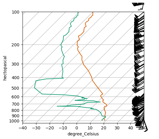
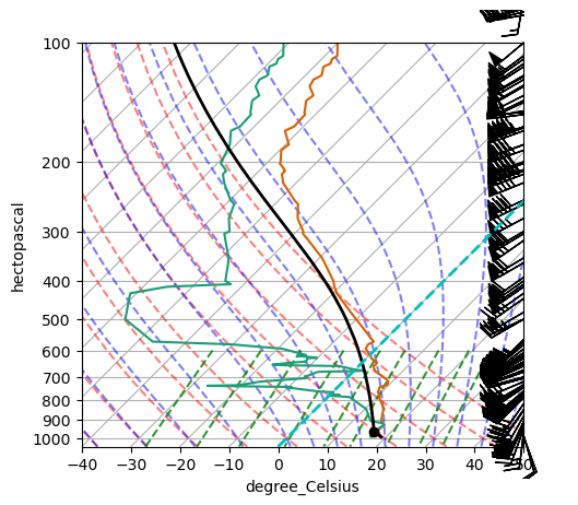
fig = plt.figure()

skew = SkewT(fig, rotation=45)

skew.plot(p, t, color=orangeish)
skew.plot(p, td, color=greenish)

skew.plot_barbs(p, u , v)

lcl_pressure, lcl_temperature = mpcalc.lcl(p[0], t[0], td[0])
skew.plot(lcl_pressure, lcl_temperature, 'ko', markerfacecolor='black')

# Calculate full parcel profile and add to plot as black line
prof = mpcalc.parcel_profile(p, t[0], td[0]).to('degC')
skew.plot(p, prof, 'k', linewidth=2)

# An example of a slanted line at constant T -- in this case the 0
# isotherm
skew.ax.axvline(0, color='c', linestyle='--', linewidth=2)

# Add the relevant special lines
skew.plot_dry_adiabats()
skew.plot_moist_adiabats()
skew.plot_mixing_lines()
/tmp/ipykernel_3321/1653287333.py:14: UserWarning: Duplicate pressure(s) [8.7] hPa provided. Output profile includes duplicate temperatures as a result.
  prof = mpcalc.parcel_profile(p, t[0], td[0]).to('degC')
<matplotlib.collections.LineCollection at 0x7f995d2aac90>
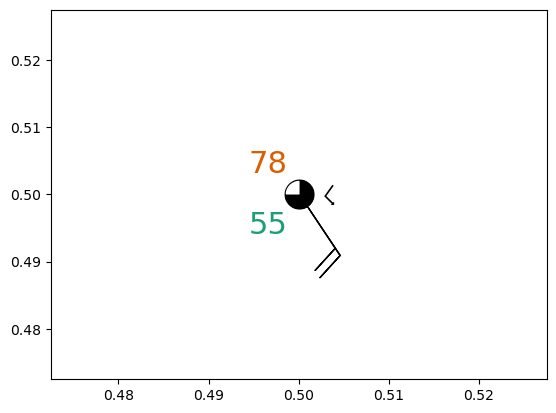
Now for something slightly different. Let’s show construction of a station plot, which we’ll use for our final plot at the end.
from metpy.plots import StationPlot, sky_cover, current_weather
fig, ax = plt.subplots()

stationplot = StationPlot(ax, 0.5, 0.5, fontsize=22)
stationplot.plot_parameter("NW", [78], color=orangeish)
stationplot.plot_parameter("SW", [55], color=greenish)
stationplot.plot_symbol("C", [6], sky_cover)
stationplot.plot_symbol("E", [13], current_weather)
stationplot.plot_barb([-10], [15])
xarray, CF conventions, and MetPy
With the power of the internet, let’s use Siphon + Unidata’s THREDDS Data Server (TDS) at NOAA PSL to access some North American Regional Reanalysis (NARR) data.
To fully reproduce this section, you will need Siphon installed via
mamba install siphon
For today, we can make do without it installed!
from siphon.catalog import TDSCatalog
cat = TDSCatalog("https://psl.noaa.gov/thredds/catalog/Datasets/NARR/Dailies/pressure/catalog.xml")
len(cat.datasets)
3745
cat.datasets[0:10]
[air.197901.nc,
 air.197902.nc,
 air.197903.nc,
 air.197904.nc,
 air.197905.nc,
 air.197906.nc,
 air.197907.nc,
 air.197908.nc,
 air.197909.nc,
 air.197910.nc]
Let’s take a closer look at our case study period, April 2008.
[data for data in cat.datasets if "200804" in data]
['air.200804.nc',
 'hgt.200804.nc',
 'omega.200804.nc',
 'shum.200804.nc',
 'tke.200804.nc',
 'uwnd.200804.nc',
 'vwnd.200804.nc']
We won’t need all of those. With a little Python-fu (or, really, “list comprehensions”), we can trim this down one last time.
variables = [var+".200804.nc" for var in ['air', 'shum', 'uwnd', 'vwnd']]
variables
['air.200804.nc', 'shum.200804.nc', 'uwnd.200804.nc', 'vwnd.200804.nc']
The TDS gives us a variety of methods and services for accessing the underlying data.
cat.datasets["air.200804.nc"].access_urls
{'OpenDAP': 'https://psl.noaa.gov/thredds/dodsC/Datasets/NARR/Dailies/pressure/air.200804.nc',
 'HTTPServer': 'https://psl.noaa.gov/thredds/fileServer/Datasets/NARR/Dailies/pressure/air.200804.nc',
 'WCS': 'https://psl.noaa.gov/thredds/wcs/Datasets/NARR/Dailies/pressure/air.200804.nc',
 'WMS': 'https://psl.noaa.gov/thredds/wms/Datasets/NARR/Dailies/pressure/air.200804.nc',
 'NetcdfSubset': 'https://psl.noaa.gov/thredds/ncss/grid/Datasets/NARR/Dailies/pressure/air.200804.nc',
 'ISO': 'https://psl.noaa.gov/thredds/iso/Datasets/NARR/Dailies/pressure/air.200804.nc',
 'NCML': 'https://psl.noaa.gov/thredds/ncml/Datasets/NARR/Dailies/pressure/air.200804.nc',
 'UDDC': 'https://psl.noaa.gov/thredds/uddc/Datasets/NARR/Dailies/pressure/air.200804.nc'}
Let’s go get those OPeNDAP links, which we know xarray will appreciate
urls = [cat.datasets[data].access_urls["OpenDAP"] for data in variables]
urls
['https://psl.noaa.gov/thredds/dodsC/Datasets/NARR/Dailies/pressure/air.200804.nc',
 'https://psl.noaa.gov/thredds/dodsC/Datasets/NARR/Dailies/pressure/shum.200804.nc',
 'https://psl.noaa.gov/thredds/dodsC/Datasets/NARR/Dailies/pressure/uwnd.200804.nc',
 'https://psl.noaa.gov/thredds/dodsC/Datasets/NARR/Dailies/pressure/vwnd.200804.nc']
urls = ['https://psl.noaa.gov/thredds/dodsC/Datasets/NARR/Dailies/pressure/air.200804.nc',
        'https://psl.noaa.gov/thredds/dodsC/Datasets/NARR/Dailies/pressure/shum.200804.nc',
        'https://psl.noaa.gov/thredds/dodsC/Datasets/NARR/Dailies/pressure/uwnd.200804.nc',
        'https://psl.noaa.gov/thredds/dodsC/Datasets/NARR/Dailies/pressure/vwnd.200804.nc']
ds = xr.open_mfdataset(urls)
ds
/home/dcamron/mambaforge/envs/ams-open-radar-2023-dev/lib/python3.11/site-packages/xarray/conventions.py:431: SerializationWarning: variable 'air' has multiple fill values {9.96921e+36, -9.96921e+36}, decoding all values to NaN.
  new_vars[k] = decode_cf_variable(
/home/dcamron/mambaforge/envs/ams-open-radar-2023-dev/lib/python3.11/site-packages/xarray/conventions.py:431: SerializationWarning: variable 'shum' has multiple fill values {9.96921e+36, -9.96921e+36}, decoding all values to NaN.
  new_vars[k] = decode_cf_variable(
/home/dcamron/mambaforge/envs/ams-open-radar-2023-dev/lib/python3.11/site-packages/xarray/conventions.py:431: SerializationWarning: variable 'uwnd' has multiple fill values {9.96921e+36, -9.96921e+36}, decoding all values to NaN.
  new_vars[k] = decode_cf_variable(
/home/dcamron/mambaforge/envs/ams-open-radar-2023-dev/lib/python3.11/site-packages/xarray/conventions.py:431: SerializationWarning: variable 'vwnd' has multiple fill values {9.96921e+36, -9.96921e+36}, decoding all values to NaN.
  new_vars[k] = decode_cf_variable(
<xarray.Dataset>
Dimensions:            (time: 30, level: 29, y: 277, x: 349, nbnds: 2)
Coordinates:
  * time               (time) datetime64[ns] 2008-04-01 ... 2008-04-30
  * level              (level) float32 1e+03 975.0 950.0 ... 150.0 125.0 100.0
  * y                  (y) float32 0.0 3.246e+04 ... 8.927e+06 8.96e+06
  * x                  (x) float32 0.0 3.246e+04 ... 1.126e+07 1.13e+07
    lat                (y, x) float32 dask.array<chunksize=(277, 349), meta=np.ndarray>
    lon                (y, x) float32 dask.array<chunksize=(277, 349), meta=np.ndarray>
Dimensions without coordinates: nbnds
Data variables:
    Lambert_Conformal  int32 -2147483647
    time_bnds          (time, nbnds) float64 dask.array<chunksize=(30, 2), meta=np.ndarray>
    air                (time, level, y, x) float32 dask.array<chunksize=(30, 29, 277, 349), meta=np.ndarray>
    shum               (time, level, y, x) float32 dask.array<chunksize=(30, 29, 277, 349), meta=np.ndarray>
    uwnd               (time, level, y, x) float32 dask.array<chunksize=(30, 29, 277, 349), meta=np.ndarray>
    vwnd               (time, level, y, x) float32 dask.array<chunksize=(30, 29, 277, 349), meta=np.ndarray>
Attributes: (12/17)
    Conventions:                     CF-1.2
    centerlat:                       50.0
    centerlon:                       -107.0
    comments:
    institution:                     National Centers for Environmental Predi...
    latcorners:                      [ 1.000001  0.897945 46.3544   46.63433 ]
    ...                              ...
    history:                         created Fri Mar 25 10:26:27 MDT 2016 by ...
    dataset_title:                   NCEP North American Regional Reanalysis ...
    references:                      https://www.esrl.noaa.gov/psd/data/gridd...
    source:                          http://www.emc.ncep.noaa.gov/mmb/rreanl/...
    _NCProperties:                   version=2,netcdf=4.6.3,hdf5=1.10.5
DODS_EXTRA.Unlimited_Dimension: timeLet’s trim that down to just our day of interest. For today’s exercise, we want to step out of dask land to avoid some quirks of MetPy + dask. Note, you can use MetPy with dask, but you will have to learn those quirks (and we will have to erode at them with our development time!).
ds = ds.sel(time="2008-04-11")
ds.load() # to de-daskify. Be careful with this for larger datasets!
<xarray.Dataset>
Dimensions: (level: 29, y: 277, x: 349, nbnds: 2)
Coordinates:
time datetime64[ns] 2008-04-11
* level (level) float32 1e+03 975.0 950.0 ... 150.0 125.0 100.0
* y (y) float32 0.0 3.246e+04 ... 8.927e+06 8.96e+06
* x (x) float32 0.0 3.246e+04 ... 1.126e+07 1.13e+07
lat (y, x) float32 1.0 1.104 1.208 ... 46.93 46.64 46.35
lon (y, x) float32 -145.5 -145.3 -145.1 ... -2.644 -2.57
Dimensions without coordinates: nbnds
Data variables:
Lambert_Conformal int32 -2147483647
time_bnds (nbnds) float64 1.826e+06 1.826e+06
air (level, y, x) float32 297.1 297.2 297.2 ... nan nan nan
shum (level, y, x) float32 0.01619 0.01612 0.01609 ... nan nan
uwnd (level, y, x) float32 -4.334 -4.334 -4.642 ... nan nan
vwnd (level, y, x) float32 -5.029 -5.029 -4.98 ... nan nan nan
Attributes: (12/17)
Conventions: CF-1.2
centerlat: 50.0
centerlon: -107.0
comments:
institution: National Centers for Environmental Predi...
latcorners: [ 1.000001 0.897945 46.3544 46.63433 ]
... ...
history: created Fri Mar 25 10:26:27 MDT 2016 by ...
dataset_title: NCEP North American Regional Reanalysis ...
references: https://www.esrl.noaa.gov/psd/data/gridd...
source: http://www.emc.ncep.noaa.gov/mmb/rreanl/...
_NCProperties: version=2,netcdf=4.6.3,hdf5=1.10.5
DODS_EXTRA.Unlimited_Dimension: timeCheck out the MetPy + xarray tutorial on our documentation, but here’s an introduction to the .metpy accessor for working with xarray data.
ds["air"].metpy.vertical
<xarray.DataArray 'level' (level: 29)>
array([1000.,  975.,  950.,  925.,  900.,  875.,  850.,  825.,  800.,  775.,
        750.,  725.,  700.,  650.,  600.,  550.,  500.,  450.,  400.,  350.,
        300.,  275.,  250.,  225.,  200.,  175.,  150.,  125.,  100.],
      dtype=float32)
Coordinates:
time datetime64[ns] 2008-04-11
* level (level) float32 1e+03 975.0 950.0 925.0 ... 175.0 150.0 125.0 100.0
Attributes:
GRIB_id: 100
GRIB_name: hPa
actual_range: [1000. 100.]
axis: Z
coordinate_defines: point
long_name: Level
positive: down
standard_name: level
units: millibar
_metpy_axis: verticalds["air"].metpy.x
<xarray.DataArray 'x' (x: 349)>
array([       0.,    32463.,    64926., ..., 11232200., 11264660., 11297120.],
      dtype=float32)
Coordinates:
time datetime64[ns] 2008-04-11
* x (x) float32 0.0 3.246e+04 6.493e+04 ... 1.126e+07 1.13e+07
Attributes:
long_name: eastward distance from southwest corner of domain in proj...
standard_name: projection_x_coordinate
units: m
_metpy_axis: xds["air"].metpy.sel(vertical=650 * units.hPa,
x=600 * units.km,
y=400000 * units.m,
method="nearest")
<xarray.DataArray 'air' ()>
array(276.60437, dtype=float32)
Coordinates:
    time     datetime64[ns] 2008-04-11
    level    float32 650.0
    y        float32 3.896e+05
    x        float32 5.843e+05
    lat      float32 5.175
    lon      float32 -143.3
Attributes: (12/14)
    GRIB_id:        11
    GRIB_name:      TMP
    grid_mapping:   Lambert_Conformal
    level_desc:     Pressure Levels
    standard_name:  air_temperature
    units:          degK
    ...             ...
    dataset:        NARR Daily Averages
    long_name:      Daily Air Temperature on Pressure Levels
    parent_stat:    Individual Obs
    statistic:      Mean
    actual_range:   [190.62566 312.67166]
_ChunkSizes: [ 1 1 277 349]We can revisit our old friend units here, too.
ds["air"].metpy.units
ds["air"].metpy.convert_units("degC")
<xarray.DataArray 'air' (level: 29, y: 277, x: 349)>
<Quantity([[[ 23.965546  24.000702  24.008514 ...        nan        nan        nan]
  [ 23.926483  23.957733  23.979218 ...        nan        nan        nan]
  [ 23.822968  23.852264  23.88742  ...        nan        nan        nan]
  ...
  [       nan        nan        nan ...        nan        nan        nan]
  [       nan        nan        nan ...        nan        nan        nan]
  [       nan        nan        nan ...        nan        nan        nan]]

 [[ 21.999115  22.024506  22.018646 ...        nan        nan        nan]
  [ 21.934662  21.9581    21.962006 ...        nan        nan        nan]
  [ 21.825287  21.805756  21.835052 ...        nan        nan        nan]
  ...
  [       nan        nan        nan ...        nan        nan        nan]
  [       nan        nan        nan ...        nan        nan        nan]
  [       nan        nan        nan ...        nan        nan        nan]]

 [[ 20.197601  20.213226  20.211273 ...        nan        nan        nan]
  [ 20.144867  20.148773  20.17807  ...        nan        nan        nan]
  [ 20.066742  20.055023  20.080414 ...        nan        nan        nan]
  ...
...
  ...
  [       nan        nan        nan ...        nan        nan        nan]
  [       nan        nan        nan ...        nan        nan        nan]
  [       nan        nan        nan ...        nan        nan        nan]]

 [[-72.83017  -72.7872   -72.754    ...        nan        nan        nan]
  [-72.808685 -72.76767  -72.73447  ...        nan        nan        nan]
  [-72.79111  -72.752045 -72.71884  ...        nan        nan        nan]
  ...
  [       nan        nan        nan ...        nan        nan        nan]
  [       nan        nan        nan ...        nan        nan        nan]
  [       nan        nan        nan ...        nan        nan        nan]]

 [[-77.892395 -77.91388  -77.93732  ...        nan        nan        nan]
  [-77.93146  -77.95685  -77.97833  ...        nan        nan        nan]
  [-77.97833  -77.99982  -78.017395 ...        nan        nan        nan]
  ...
  [       nan        nan        nan ...        nan        nan        nan]
  [       nan        nan        nan ...        nan        nan        nan]
  [       nan        nan        nan ...        nan        nan        nan]]], 'degree_Celsius')>
Coordinates:
    time     datetime64[ns] 2008-04-11
  * level    (level) float32 1e+03 975.0 950.0 925.0 ... 175.0 150.0 125.0 100.0
  * y        (y) float32 0.0 3.246e+04 6.493e+04 ... 8.927e+06 8.96e+06
  * x        (x) float32 0.0 3.246e+04 6.493e+04 ... 1.126e+07 1.13e+07
    lat      (y, x) float32 1.0 1.104 1.208 1.312 ... 47.22 46.93 46.64 46.35
    lon      (y, x) float32 -145.5 -145.3 -145.1 -144.9 ... -2.718 -2.644 -2.57
Attributes: (12/13)
    GRIB_id:        11
    GRIB_name:      TMP
    grid_mapping:   Lambert_Conformal
    level_desc:     Pressure Levels
    standard_name:  air_temperature
    valid_range:    [137.5 362.5]
    ...             ...
    dataset:        NARR Daily Averages
    long_name:      Daily Air Temperature on Pressure Levels
    parent_stat:    Individual Obs
    statistic:      Mean
    actual_range:   [190.62566 312.67166]
_ChunkSizes: [ 1 1 277 349]If you’re working with data that follow the Climate and Forecasting (CF) Metadata Conventions, MetPy can understand that metadata and make it more Python friendly for you.
ds = ds.metpy.parse_cf()
ds
<xarray.Dataset>
Dimensions:            (nbnds: 2, level: 29, y: 277, x: 349)
Coordinates:
    time               datetime64[ns] 2008-04-11
  * level              (level) float32 1e+03 975.0 950.0 ... 150.0 125.0 100.0
  * y                  (y) float32 0.0 3.246e+04 ... 8.927e+06 8.96e+06
  * x                  (x) float32 0.0 3.246e+04 ... 1.126e+07 1.13e+07
    lat                (y, x) float32 1.0 1.104 1.208 ... 46.93 46.64 46.35
    lon                (y, x) float32 -145.5 -145.3 -145.1 ... -2.644 -2.57
    metpy_crs          object Projection: lambert_conformal_conic
Dimensions without coordinates: nbnds
Data variables:
    Lambert_Conformal  int32 -2147483647
    time_bnds          (nbnds) float64 1.826e+06 1.826e+06
    air                (level, y, x) float32 297.1 297.2 297.2 ... nan nan nan
    shum               (level, y, x) float32 0.01619 0.01612 0.01609 ... nan nan
    uwnd               (level, y, x) float32 -4.334 -4.334 -4.642 ... nan nan
    vwnd               (level, y, x) float32 -5.029 -5.029 -4.98 ... nan nan nan
Attributes: (12/17)
    Conventions:                     CF-1.2
    centerlat:                       50.0
    centerlon:                       -107.0
    comments:
    institution:                     National Centers for Environmental Predi...
    latcorners:                      [ 1.000001  0.897945 46.3544   46.63433 ]
    ...                              ...
    history:                         created Fri Mar 25 10:26:27 MDT 2016 by ...
    dataset_title:                   NCEP North American Regional Reanalysis ...
    references:                      https://www.esrl.noaa.gov/psd/data/gridd...
    source:                          http://www.emc.ncep.noaa.gov/mmb/rreanl/...
    _NCProperties:                   version=2,netcdf=4.6.3,hdf5=1.10.5
DODS_EXTRA.Unlimited_Dimension: timeds["air"].metpy.cartopy_crs
<cartopy.crs.LambertConformal object at 0x7f995de45590>
We’ll take a step back to select across our entire dataset for some calculations.
ds = ds.sel(level=650)
mpcalc.dewpoint_from_specific_humidity?
Signature:
mpcalc.dewpoint_from_specific_humidity(
    pressure,
    temperature,
    specific_humidity,
)
Docstring:
Calculate the dewpoint from specific humidity, temperature, and pressure.

Parameters
----------
pressure: `pint.Quantity`
    Total atmospheric pressure

temperature: `pint.Quantity`
    Air temperature

specific_humidity: `pint.Quantity`
    Specific humidity of air

Returns
-------
`pint.Quantity`
    Dew point temperature

Examples
--------
>>> from metpy.calc import dewpoint_from_specific_humidity
>>> from metpy.units import units
>>> dewpoint_from_specific_humidity(1000 * units.hPa, 10 * units.degC, 5 * units('g/kg'))
<Quantity(3.73203192, 'degree_Celsius')>

.. versionchanged:: 1.0
   Changed signature from ``(specific_humidity, temperature, pressure)``

See Also
--------
relative_humidity_from_mixing_ratio, dewpoint_from_relative_humidity
File:      ~/mambaforge/envs/ams-open-radar-2023-dev/lib/python3.11/site-packages/metpy/calc/thermo.py
Type:      function
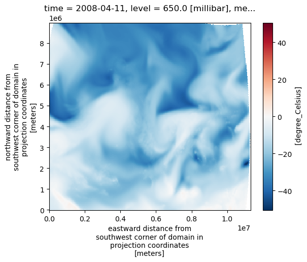
dewpoint = mpcalc.dewpoint_from_specific_humidity(ds.level, ds.air, ds.shum)
dewpoint
<xarray.DataArray (y: 277, x: 349)>
<Quantity([[-7.7446594 -7.754944  -7.762787  ...        nan        nan        nan]
 [-7.70578   -7.711151  -7.721405  ...        nan        nan        nan]
 [-7.6646423 -7.669464  -7.6772156 ...        nan        nan        nan]
 ...
 [       nan        nan        nan ...        nan        nan        nan]
 [       nan        nan        nan ...        nan        nan        nan]
 [       nan        nan        nan ...        nan        nan        nan]], 'degree_Celsius')>
Coordinates:
    time       datetime64[ns] 2008-04-11
    level      float32 650.0
  * y          (y) float32 0.0 3.246e+04 6.493e+04 ... 8.927e+06 8.96e+06
  * x          (x) float32 0.0 3.246e+04 6.493e+04 ... 1.126e+07 1.13e+07
    lat        (y, x) float32 1.0 1.104 1.208 1.312 ... 47.22 46.93 46.64 46.35
    lon        (y, x) float32 -145.5 -145.3 -145.1 ... -2.718 -2.644 -2.57
metpy_crs object Projection: lambert_conformal_conicdewpoint.plot()
<matplotlib.collections.QuadMesh at 0x7f995de5f8d0>
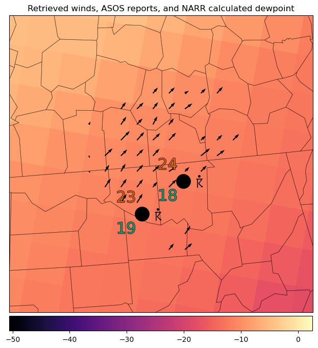
Putting it all together
khtx_file = "../pydda/output_grid_KHTX.nc"
armor_file = "../pydda/output_grid_ARMOR.nc"
khtx_ds = pyart.io.read_grid(khtx_file).to_xarray().sel(z=3000).squeeze()
armor_ds = pyart.io.read_grid(armor_file).to_xarray().sel(z=3000).squeeze()
/home/dcamron/mambaforge/envs/ams-open-radar-2023-dev/lib/python3.11/site-packages/pyart/io/cfradial.py:408: UserWarning: WARNING: valid_min not used since it
cannot be safely cast to variable data type
  data = self.ncvar[:]
/home/dcamron/mambaforge/envs/ams-open-radar-2023-dev/lib/python3.11/site-packages/pyart/io/cfradial.py:408: UserWarning: WARNING: valid_max not used since it
cannot be safely cast to variable data type
  data = self.ncvar[:]
from metpy.plots import USCOUNTIES
from matplotlib.patheffects import withStroke

# Setting up our figure and desired map projection with Cartopy
fig, ax = plt.subplots(figsize=(9, 9), subplot_kw={"projection": ccrs.LambertConformal()})

ax.set_extent((-88, -85.5, 34, 36), crs=ccrs.PlateCarree())

# Starting with our calculated dewpoint from remotely accessed NARR data
cf = ax.pcolormesh(dewpoint.metpy.x, dewpoint.metpy.y, dewpoint,
                 transform=dewpoint.metpy.cartopy_crs, cmap="magma")

# Plot our PyDDA retrieved winds from KHTX and ARMOR as quivers
ax.quiver(khtx_ds.lon.data, khtx_ds.lat.data,
          khtx_ds.u.data, khtx_ds.v.data,
          transform=ccrs.PlateCarree(),
          regrid_shape=20)

ax.quiver(armor_ds.lon.data, armor_ds.lat.data,
          armor_ds.u.data, armor_ds.v.data,
          transform=ccrs.PlateCarree(),
          regrid_shape=20)

# Include DCU and MDQ ASOS reports as station plots with
# temperature, dewpoint, cloud cover, and current weather reports
stationplot = StationPlot(ax, subset["longitude"], subset["latitude"],
                          transform=ccrs.PlateCarree(), clip_on=True, fontsize=22)

stationplot.plot_parameter("NW", subset["air_temperature"], color=orangeish,
                           path_effects=[withStroke(linewidth=1, foreground="black")])
stationplot.plot_parameter("SW", subset["dew_point_temperature"],color=greenish,
                           path_effects=[withStroke(linewidth=1, foreground="black")])
stationplot.plot_symbol("C", subset["cloud_coverage"], sky_cover)
stationplot.plot_symbol("E", subset["current_wx1_symbol"], current_weather)

# Use Cartopy + MetPy for county outlines, helpful at this scale
ax.add_feature(USCOUNTIES, alpha=0.5, linewidth=0.5)

# Some final touching up, and...
fig.colorbar(cf, orientation="horizontal", pad=0.01, shrink=0.852)

ax.set_title("""Retrieved winds, ASOS reports, and NARR calculated dewpoint""")
Text(0.5, 1.0, 'Retrieved winds, ASOS reports, and NARR calculated dewpoint')
Downloading file 'us_counties_20m.dbf' from 'https://github.com/Unidata/MetPy/raw/v1.5.1/staticdata/us_counties_20m.dbf' to '/home/dcamron/.cache/metpy/v1.5.1'.
Downloading file 'us_counties_20m.shx' from 'https://github.com/Unidata/MetPy/raw/v1.5.1/staticdata/us_counties_20m.shx' to '/home/dcamron/.cache/metpy/v1.5.1'.
Downloading file 'us_counties_20m.shp' from 'https://github.com/Unidata/MetPy/raw/v1.5.1/staticdata/us_counties_20m.shp' to '/home/dcamron/.cache/metpy/v1.5.1'.
Resources and references
MetPy Cookbook (under construction, contribute today!)