PyDDA tutorial
![]()
PyDDA is an open source Python package for retrieving winds using Multiple Doppler analyses. It uses the 3D variational technique for retrieving winds from multiple Doppler radars. It uses Py-ART Grid Objects as inputs. Therefore, preprocessed and gridded data are needed for PyDDA to run.
3D variational technique
PyDDA uses a 3D variational technique to retrieve the 3D wind field. We will leave students that are interested in more information about these technqiues two references to read at the end of this notebook. A basic introduction to 3D variational analysis is given here.
PyDDA minimizes a cost function \(J\) that corresponds to various penalties including:
\(J_{m} = \nabla \cdot V\) which corresponds to the mass continuity equation.
\(J_{o} = \) RMSE between radar winds and analysis winds.
\(J_{b} = \) RMSE between sounding winds and analysis winds.
\(J_{s} = \nabla^2 V\) which corresponds to the smoothness of wind field to eliminate high-frequency noise that can result from numerical instability.
The cost function to be minimized is a weighted sum of the various cost functions in PyDDA and are represented in Equation (1):
$J = c_{m}J_{m} + c_{o}J_{o} + c_{b}J_{b} + c_{s}J_{s} + ...$ (1)
Imports
Let’s import the necessary libraries. For now, we’ll need PyART, glob, matplotlib, and PyDDA.
import glob
import fsspec

import pyart
import matplotlib.pyplot as plt
import pydda
import warnings
import numpy as np
import pandas as pd
import cartopy.crs as ccrs
warnings.filterwarnings("ignore")
## You are using the Python ARM Radar Toolkit (Py-ART), an open source
## library for working with weather radar data. Py-ART is partly
## supported by the U.S. Department of Energy as part of the Atmospheric
## Radiation Measurement (ARM) Climate Research Facility, an Office of
## Science user facility.
##
## If you use this software to prepare a publication, please cite:
##
##     JJ Helmus and SM Collis, JORS 2016, doi: 10.5334/jors.119
2023-07-27 14:13:08.262546: I tensorflow/core/platform/cpu_feature_guard.cc:193] This TensorFlow binary is optimized with oneAPI Deep Neural Network Library (oneDNN) to use the following CPU instructions in performance-critical operations:  SSE4.1 SSE4.2 AVX AVX2 AVX512F AVX512_VNNI FMA
To enable them in other operations, rebuild TensorFlow with the appropriate compiler flags.
Welcome to PyDDA 1.3.1
Detecting Jax...
Jax engine enabled!
Detecting TensorFlow...
TensorFlow detected. Checking for tensorflow-probability...
TensorFlow-probability detected. TensorFlow engine enabled!
Case study
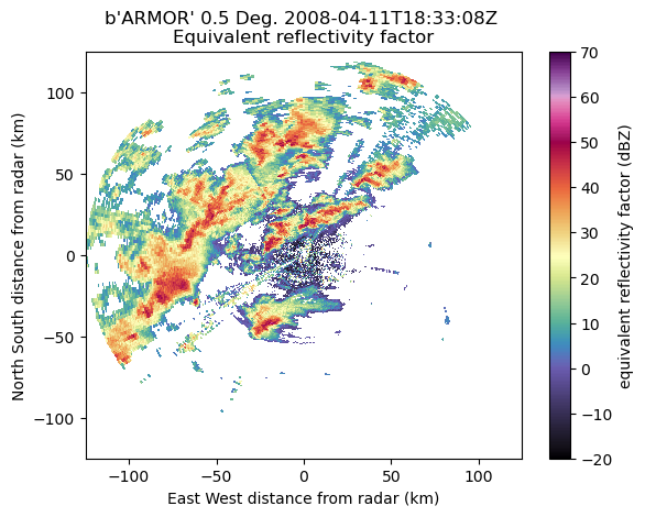
We will examine the same case study over Northern Alabama that has been used for this entire short course. For this case in April 2008, we had an MCS with supercells out ahead of the main line approach the Huntsville, AL region. 3D variational retrievals of thunderstorm updrafts can have uncertainties on the order of 5 m/s. In addition these retrievals require precipitation coverage throughout the domain. Therefore, 3DVAR retrievals are best suited for deep convection like this where the updrafts are strong and precipitation coverage is wide.
For this case, we had coverage of the storm from two radars, the ARMOR and the Huntsville NEXRAD radar.
UAH ARMOR Radar
We need to load and preprocess the UAH armor data first. In order to do so, we first need to load the ARMOR radar file.
files = glob.glob('../../data/uah-armor/RAW_NA_*')
radar = pyart.io.read(files[1])
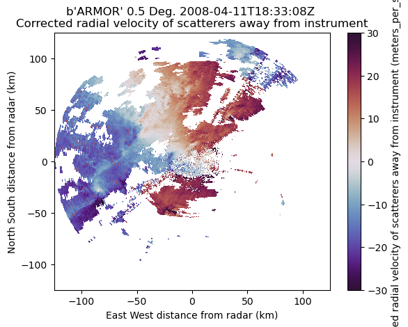
Dealiasing
The next step is to dealias the radar data. We will follow the steps that were shown eariler in this course to dealias the radar data.
nyquist = radar.instrument_parameters['nyquist_velocity']['data'][0]
vel_dealias = pyart.correct.dealias_region_based(radar,
                                                    vel_field='velocity',
                                                    nyquist_vel=nyquist,
                                                    centered=True,
                                                    )
radar.add_field('corrected_velocity', vel_dealias, replace_existing=True)
Plot the data to make sure dealiasing succeeded.
display = pyart.graph.RadarDisplay(radar)
display.plot('reflectivity',
             vmin=-20,
             vmax=70,
             cmap='pyart_ChaseSpectral',
             sweep=0)
display = pyart.graph.RadarDisplay(radar)
display.plot('corrected_velocity',
             vmin=-30,
             vmax=30,
             cmap='twilight_shifted',
             sweep=0)
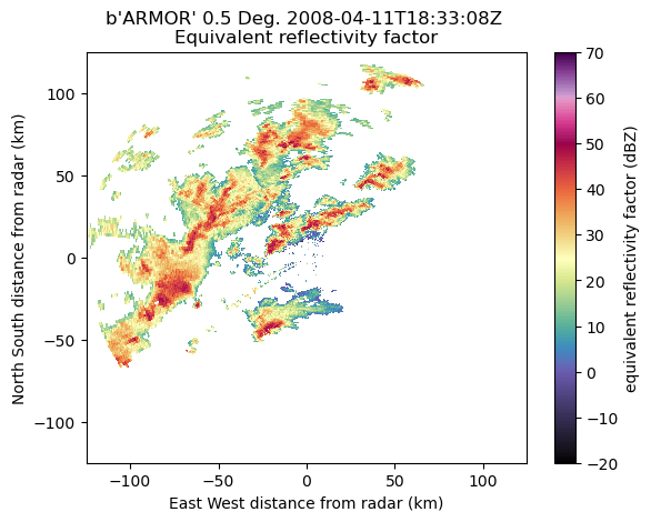
Let’s despeckle the above radar data to remove some artifacts.
gatefilter = pyart.filters.GateFilter(radar)
gatefilter.exclude_above('spectrum_width', 7)
gatefilter.exclude_below('cross_correlation_ratio', 0.8)
gatefilter = pyart.correct.despeckle_field(radar, 'reflectivity', gatefilter=gatefilter)
display = pyart.graph.RadarDisplay(radar)
display.plot('reflectivity',
             vmin=-20,
             vmax=70, gatefilter=gatefilter,
             cmap='pyart_ChaseSpectral',
             sweep=0)
Gridding
PyDDA requires data to be gridded to Cartesian coordinates in order to retrieve the 3D wind fields. Therefore, we will use Py-ART’s grid_from_radars function in order to do the gridding. You usually want to have a grid resolution such that your features of interest are covered by four grid points. In this case, we’re at 1 km horizontal and 0.5 km vertical resolution. For more information on gridding with Py-ART, see the Radar Cookbook.
grid_limits = ((0., 15000.), (-100_000., 100_000.), (-100_000., 100_000.))
grid_shape = (31, 201, 201)
radar.fields["corrected_velocity"]["data"] = np.ma.masked_where(gatefilter.gate_excluded,
                                                        radar.fields["corrected_velocity"]["data"])
radar.fields["reflectivity"]["data"] = np.ma.masked_where(gatefilter.gate_excluded,
                                                        radar.fields["reflectivity"]["data"])

uah_grid = pyart.map.grid_from_radars([radar], grid_limits=grid_limits,
                                 grid_shape=grid_shape)
uah_ds = uah_grid.to_xarray()
uah_ds
<xarray.Dataset>
Dimensions:                      (time: 1, z: 31, y: 201, x: 201)
Coordinates:
  * time                         (time) object 2008-04-11 18:33:08
  * z                            (z) float64 0.0 500.0 ... 1.45e+04 1.5e+04
    lat                          (y, x) float64 33.74 33.74 ... 35.54 35.54
    lon                          (y, x) float64 -87.85 -87.84 ... -85.68 -85.67
  * y                            (y) float64 -1e+05 -9.9e+04 ... 9.9e+04 1e+05
  * x                            (x) float64 -1e+05 -9.9e+04 ... 9.9e+04 1e+05
Data variables:
    specific_differential_phase  (time, z, y, x) float32 nan nan nan ... nan nan
    total_power                  (time, z, y, x) float32 nan nan nan ... nan nan
    cross_correlation_ratio      (time, z, y, x) float32 nan nan nan ... nan nan
    reflectivity                 (time, z, y, x) float32 nan nan nan ... nan nan
    velocity                     (time, z, y, x) float32 nan nan nan ... nan nan
    spectrum_width               (time, z, y, x) float32 nan nan nan ... nan nan
    differential_reflectivity    (time, z, y, x) float32 nan nan nan ... nan nan
    corrected_velocity           (time, z, y, x) float32 nan nan nan ... nan nan
    differential_phase           (time, z, y, x) float32 nan nan nan ... nan nan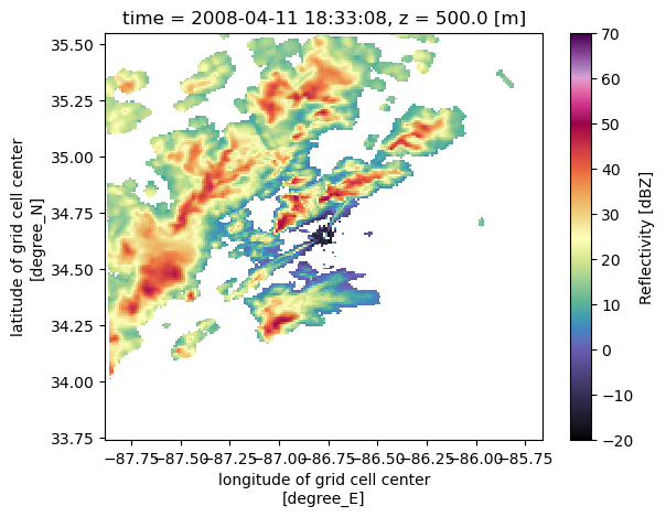
ROI (time, z, y, x) float32 3.703e+03 ... 4.453e+03Let’s make sure the grid looks good!
uah_ds.isel(z=1).reflectivity.plot(x='lon',
                                   y='lat',
                                   vmin=-20,
                                   vmax=70,
                                   cmap='pyart_ChaseSpectral')
<matplotlib.collections.QuadMesh at 0x17c63b040>
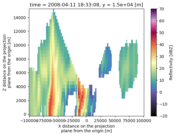
uah_ds.isel(y=115).reflectivity.plot(x='x',
                                   y='z',
                                   vmin=-20,
                                   vmax=70,
                                   cmap='pyart_ChaseSpectral')
<matplotlib.collections.QuadMesh at 0x17c3c4ac0>
NEXRAD Data
Next, we need to load the NEXRAD data. This is available on Amazon Web Services under the noaa-nexrad-level2 bucket. This S3 bucket has all of the historical NEXRAD WSR-88D level 2 data that is available for the continential US Use the below code snippet to retrieve the NEXRAD data from Amazon Web Services.
fs = fsspec.filesystem("s3", anon=True)
files = sorted(fs.glob("s3://noaa-nexrad-level2/2008/04/11/KHTX/KHTX20080411_18*"))
files
['noaa-nexrad-level2/2008/04/11/KHTX/KHTX20080411_180040.gz',
 'noaa-nexrad-level2/2008/04/11/KHTX/KHTX20080411_180647.gz',
 'noaa-nexrad-level2/2008/04/11/KHTX/KHTX20080411_181144.gz',
 'noaa-nexrad-level2/2008/04/11/KHTX/KHTX20080411_181643.gz',
 'noaa-nexrad-level2/2008/04/11/KHTX/KHTX20080411_182140.gz',
 'noaa-nexrad-level2/2008/04/11/KHTX/KHTX20080411_182639.gz',
 'noaa-nexrad-level2/2008/04/11/KHTX/KHTX20080411_183137.gz',
 'noaa-nexrad-level2/2008/04/11/KHTX/KHTX20080411_183635.gz',
 'noaa-nexrad-level2/2008/04/11/KHTX/KHTX20080411_184134.gz',
 'noaa-nexrad-level2/2008/04/11/KHTX/KHTX20080411_184632.gz',
 'noaa-nexrad-level2/2008/04/11/KHTX/KHTX20080411_185130.gz',
 'noaa-nexrad-level2/2008/04/11/KHTX/KHTX20080411_185628.gz']
Read a single file, the one closes to the UAH volume scan used before
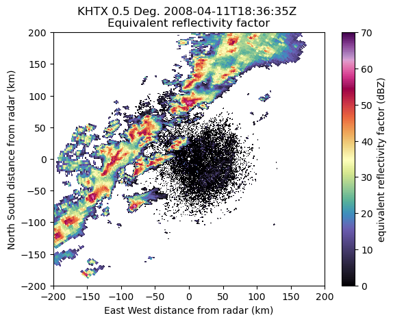
nexrad_radar = pyart.io.read_nexrad_archive(f's3://{files[7]}', station='KHTX')
Visualize the data to make sure we have the correct scan.
display = pyart.graph.RadarDisplay(nexrad_radar)
display.plot('reflectivity',
                     vmin=0,
                     vmax=70,
                     cmap='pyart_ChaseSpectral',
                     sweep=0)
plt.ylim(-200, 200)
plt.xlim(-200, 200)
(-200.0, 200.0)
The NEXRAD level 2 also need to be dealiased. We will still need to filter out the noise in the above radar data.
# Use the ARMOR radar lat/lon as the center for the grid
grid_lat = radar.latitude['data'][0]
grid_lon = radar.longitude['data'][0]
vel_dealias = pyart.correct.dealias_region_based(nexrad_radar,
                                                    vel_field='velocity',
                                                    nyquist_vel=nyquist,
                                                    centered=True,
                                                    )
nexrad_radar.add_field('corrected_velocity', vel_dealias, replace_existing=True)


nexrad_grid = pyart.map.grid_from_radars([nexrad_radar],
                                         grid_limits=grid_limits,
                                         grid_shape=grid_shape,
                                         grid_origin=(grid_lat, grid_lon),
                                        )

# Convert to xarray and remove the time dimension
nexrad_ds = nexrad_grid.to_xarray().squeeze()
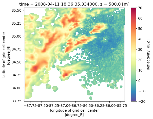
Visualize the grids
Let’s see what our output data looks like!
nexrad_ds.reflectivity.isel(z=1).plot(x='lon',
                                      y='lat',
                                      cmap='Spectral_r',
                                      vmin=-20,
                                      vmax=70)
<matplotlib.collections.QuadMesh at 0x17ebe3c70>
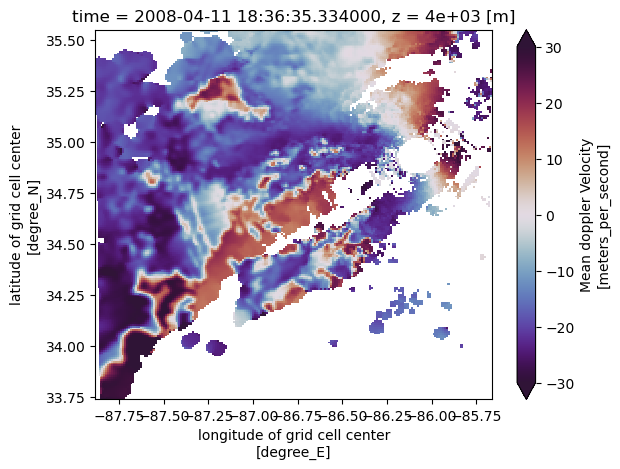
nexrad_ds.velocity.isel(z=8).plot(x='lon',
                                  y='lat',
                                  cmap='twilight_shifted',
                                  vmin=-30,
                                  vmax=30)
<matplotlib.collections.QuadMesh at 0x17c8e6890>
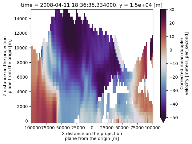
nexrad_ds.corrected_velocity.isel(y=115).plot(x='x',
                                  y='z',
                                  cmap='twilight_shifted',
                                  vmin=-50,
                                  vmax=30)
<matplotlib.collections.QuadMesh at 0x17dba1900>
PyDDA initialization
The 3DVAR wind retrieval first requires an initial guess at the wind field in order to start the cost function minimization process. PyDDA has support for using WRF and sounding data as an initial guess of the wind field as well as constant wind fields.
Initalization functions in pydda.initialization module: |
Functionality |
|---|---|
make_constant_wind_field(Grid[, wind, vel_field]) |
This function makes a constant wind field given a wind vector |
make_wind_field_from_profile(Grid, profile) |
This function makes a 3D wind field from a sounding. |
make_background_from_wrf(Grid, file_path, …) |
This function makes an initalization field based off of the u and w from a WRF run. |
make_initialization_from_era_interim(Grid[, …]) |
This function will read ERA Interim in NetCDF format and add it to the Py-ART grid specified by Grid. |
For this example, we will use the closest NWS Sounding present in time as an initialization. The initial state is extremely important for the retrieval. If you specify a zero initial state, this has a tendency to have PyDDA resolve false updrafts and downdrafts in the cone of silence as the optimization loop will hold the background state to be zero where there is no radar data. Specifying the initial state, or a background constraint, will specify what the winds should be outside of the region of data coverage.
The bottom code snippet will load a University of Wyoming sounding file, remove the NaNs, then convert the
col_names = ["PRES", "HGHT", "TEMP", "DWPT", "RELH", "MIXR", "DRCT", "SKNT", "THTA", "THTE", "THTV"]
sounding = pd.read_csv(
    '../../data/sounding_data/bmx_sounding_20080411_12Z.txt',
    skiprows=4, names=col_names, delimiter='\s+')
spd = sounding["SKNT"]*0.5144

u_back = -spd * np.sin(np.deg2rad(sounding["DRCT"]))
v_back = -spd * np.cos(np.deg2rad(sounding["DRCT"]))
z_back = sounding["HGHT"]
# Remove NaNs from profile
isnan = np.logical_or.reduce((~np.isfinite(u_back), ~np.isfinite(v_back), ~np.isfinite(z_back)))
u_back = u_back[~isnan]
v_back = v_back[~isnan]
z_back = z_back[~isnan]
spd = spd[~isnan]
drct = sounding["DRCT"][~isnan]
profile = pyart.core.HorizontalWindProfile(sounding["HGHT"][~isnan], spd, drct)
uah_grid = pydda.initialization.make_wind_field_from_profile(
    uah_grid, profile)
PyDDA wind retrieval
The core wind retrieval function in PyDDA is done using retrieval.get_dd_wind_field. It has many potential keyword inputs that the user can enter. In this example, we are specifying:
Input to pydda.initialization module: |
Meaning |
Value |
|---|---|---|
Grids |
The input grids to analyze. |
[uah_grid, nexrad_grid] |
u_init |
Initial guess of u field. |
u_init |
v_init |
Initial guess of u field. |
v_init |
w_init |
Initial guess of u field. |
w_init |
Co |
Weight for cost function related to radar observations |
1.0 |
Cm |
Weight of cost function related to mass continuity equation |
256.0 |
Cx |
Weight of cost function for smoothess in the x-direction |
1e-3 |
Cy |
Weight of cost function for smoothess in the y-direction |
1e-3 |
Cz |
Weight of cost function for smoothess in the z-direction |
1e-3 |
Cb |
Weight of cost function for sounding (background) constraint |
0 |
frz |
The freezing level in meters. This is to tell PyDDA where to use ice particle fall speeds in the wind retrieval verus liquid. |
5000. |
filter_window |
The window to apply the low pass filter on |
5 |
mask_outside_opt |
Mask all winds outside the Dual Doppler lobes |
True |
vel_name |
The name of the velocity field in the radar data |
‘corrected_velocity’ |
wind_tol |
Stop optimization when the change in wind speeds between iterations is less than this value |
|
engine |
PyDDA supports three backends for optimization: SciPy, JAX, and TensorFlow. |
“scipy” |
grids, params = pydda.retrieval.get_dd_wind_field([uah_grid, nexrad_grid],
                                                  Co=0.1, Cm=1024.,
                                                  Cx=1e2, Cy=1e2, Cz=1e2, Cb=0,
                                                  frz=5000.0, filter_window=5,
                                                  mask_outside_opt=True, upper_bc=1,
                                                  vel_name='corrected_velocity',
                                                  wind_tol=0.5, engine="scipy")
Calculating weights for radars 0 and 1
Calculating weights for radars 1 and 0
Calculating weights for models...
Starting solver
rmsVR = 20.876722950399113
Total points: 442768
The max of w_init is 0.0
Nfeval | Jvel    | Jmass   | Jsmooth |   Jbg   | Jvort   | Jmodel  | Jpoint  | Max w
      0|7760.2314|   0.0000|   0.0000|   0.0000|   0.0000|   0.0000|   0.0000|   0.0000
The gradient of the cost functions is 13.07816872627942
Nfeval | Jvel    | Jmass   | Jsmooth |   Jbg   | Jvort   | Jmodel  | Jpoint  | Max w
     10|3193.7016| 182.9802|   0.0002|   0.0000|   0.0000|   0.0000|   0.0000|  12.8805
The gradient of the cost functions is 13.105214307953752
Nfeval | Jvel    | Jmass   | Jsmooth |   Jbg   | Jvort   | Jmodel  | Jpoint  | Max w
     20|3193.4959| 183.0661|   0.0002|   0.0000|   0.0000|   0.0000|   0.0000|  12.8848
The gradient of the cost functions is 6.019453585457773
Nfeval | Jvel    | Jmass   | Jsmooth |   Jbg   | Jvort   | Jmodel  | Jpoint  | Max w
     30|2697.2148|  83.3260|   0.0001|   0.0000|   0.0000|   0.0000|   0.0000|   6.7618
Max change in w: 7.275
The gradient of the cost functions is 2.2243440012501026
Nfeval | Jvel    | Jmass   | Jsmooth |   Jbg   | Jvort   | Jmodel  | Jpoint  | Max w
     40|1540.5529|  91.7874|   0.0002|   0.0000|   0.0000|   0.0000|   0.0000|   9.0003
Max change in w: 5.134
The gradient of the cost functions is 1.4422257081703
Nfeval | Jvel    | Jmass   | Jsmooth |   Jbg   | Jvort   | Jmodel  | Jpoint  | Max w
     50| 867.7180|  99.2598|   0.0002|   0.0000|   0.0000|   0.0000|   0.0000|  11.0569
Max change in w: 1.933
The gradient of the cost functions is 0.9386451567759319
Nfeval | Jvel    | Jmass   | Jsmooth |   Jbg   | Jvort   | Jmodel  | Jpoint  | Max w
     60| 574.8696|  84.6962|   0.0002|   0.0000|   0.0000|   0.0000|   0.0000|  11.6313
Max change in w: 3.236
The gradient of the cost functions is 1.4722537569315763
Nfeval | Jvel    | Jmass   | Jsmooth |   Jbg   | Jvort   | Jmodel  | Jpoint  | Max w
     70| 473.3045|  81.3971|   0.0002|   0.0000|   0.0000|   0.0000|   0.0000|  12.2525
Max change in w: 1.903
The gradient of the cost functions is 1.2149815684084517
Nfeval | Jvel    | Jmass   | Jsmooth |   Jbg   | Jvort   | Jmodel  | Jpoint  | Max w
     80| 399.0485|  77.5946|   0.0002|   0.0000|   0.0000|   0.0000|   0.0000|  13.1615
Max change in w: 1.989
The gradient of the cost functions is 0.3997606378071222
Nfeval | Jvel    | Jmass   | Jsmooth |   Jbg   | Jvort   | Jmodel  | Jpoint  | Max w
     90| 366.5867|  72.6215|   0.0002|   0.0000|   0.0000|   0.0000|   0.0000|  13.5110
Max change in w: 2.098
The gradient of the cost functions is 0.4521480861324039
Nfeval | Jvel    | Jmass   | Jsmooth |   Jbg   | Jvort   | Jmodel  | Jpoint  | Max w
    100| 339.5158|  65.0863|   0.0002|   0.0000|   0.0000|   0.0000|   0.0000|  13.6459
Max change in w: 2.118
The gradient of the cost functions is 0.6312901575204206
Nfeval | Jvel    | Jmass   | Jsmooth |   Jbg   | Jvort   | Jmodel  | Jpoint  | Max w
    110| 317.5584|  63.1234|   0.0002|   0.0000|   0.0000|   0.0000|   0.0000|  13.9376
Max change in w: 3.110
The gradient of the cost functions is 0.25010558921884835
Nfeval | Jvel    | Jmass   | Jsmooth |   Jbg   | Jvort   | Jmodel  | Jpoint  | Max w
    120| 297.3736|  63.0243|   0.0002|   0.0000|   0.0000|   0.0000|   0.0000|  14.2744
Max change in w: 1.445
The gradient of the cost functions is 0.27626134250579887
Nfeval | Jvel    | Jmass   | Jsmooth |   Jbg   | Jvort   | Jmodel  | Jpoint  | Max w
    130| 289.2224|  59.8914|   0.0002|   0.0000|   0.0000|   0.0000|   0.0000|  14.9319
Max change in w: 1.604
The gradient of the cost functions is 0.38603660071829865
Nfeval | Jvel    | Jmass   | Jsmooth |   Jbg   | Jvort   | Jmodel  | Jpoint  | Max w
    140| 283.3340|  58.7634|   0.0002|   0.0000|   0.0000|   0.0000|   0.0000|  15.8898
Max change in w: 2.107
The gradient of the cost functions is 0.2654674447612781
Nfeval | Jvel    | Jmass   | Jsmooth |   Jbg   | Jvort   | Jmodel  | Jpoint  | Max w
    150| 277.4301|  58.0832|   0.0002|   0.0000|   0.0000|   0.0000|   0.0000|  16.5992
Max change in w: 1.326
The gradient of the cost functions is 0.25161315135570883
Nfeval | Jvel    | Jmass   | Jsmooth |   Jbg   | Jvort   | Jmodel  | Jpoint  | Max w
    160| 274.3603|  56.0786|   0.0002|   0.0000|   0.0000|   0.0000|   0.0000|  17.0818
The gradient of the cost functions is 0.1878580225897227
Nfeval | Jvel    | Jmass   | Jsmooth |   Jbg   | Jvort   | Jmodel  | Jpoint  | Max w
    170| 275.1130|  54.6835|   0.0002|   0.0000|   0.0000|   0.0000|   0.0000|  17.6231
Max change in w: 1.283
The gradient of the cost functions is 0.2028893528222265
Nfeval | Jvel    | Jmass   | Jsmooth |   Jbg   | Jvort   | Jmodel  | Jpoint  | Max w
    180| 275.3288|  52.8382|   0.0002|   0.0000|   0.0000|   0.0000|   0.0000|  18.8000
Max change in w: 1.427
The gradient of the cost functions is 0.27150836378235566
Nfeval | Jvel    | Jmass   | Jsmooth |   Jbg   | Jvort   | Jmodel  | Jpoint  | Max w
    190| 273.4343|  52.0998|   0.0002|   0.0000|   0.0000|   0.0000|   0.0000|  20.1749
Max change in w: 1.385
The gradient of the cost functions is 0.6200873649489808
Nfeval | Jvel    | Jmass   | Jsmooth |   Jbg   | Jvort   | Jmodel  | Jpoint  | Max w
    200| 271.6871|  51.1359|   0.0002|   0.0000|   0.0000|   0.0000|   0.0000|  20.9883
Max change in w: 1.430
The gradient of the cost functions is 0.23838997025900646
Nfeval | Jvel    | Jmass   | Jsmooth |   Jbg   | Jvort   | Jmodel  | Jpoint  | Max w
    210| 267.1408|  51.0702|   0.0002|   0.0000|   0.0000|   0.0000|   0.0000|  22.0295
Max change in w: 1.774
The gradient of the cost functions is 0.25219322289770224
Nfeval | Jvel    | Jmass   | Jsmooth |   Jbg   | Jvort   | Jmodel  | Jpoint  | Max w
    220| 262.8213|  52.6046|   0.0002|   0.0000|   0.0000|   0.0000|   0.0000|  24.0906
Max change in w: 1.879
The gradient of the cost functions is 0.41402138195674065
Nfeval | Jvel    | Jmass   | Jsmooth |   Jbg   | Jvort   | Jmodel  | Jpoint  | Max w
    230| 261.4781|  53.6816|   0.0002|   0.0000|   0.0000|   0.0000|   0.0000|  25.1616
The gradient of the cost functions is 0.20406839195420667
Nfeval | Jvel    | Jmass   | Jsmooth |   Jbg   | Jvort   | Jmodel  | Jpoint  | Max w
    240| 261.2789|  53.8313|   0.0002|   0.0000|   0.0000|   0.0000|   0.0000|  25.3298
The gradient of the cost functions is 0.28541487637255214
Nfeval | Jvel    | Jmass   | Jsmooth |   Jbg   | Jvort   | Jmodel  | Jpoint  | Max w
    250| 261.1041|  53.9973|   0.0002|   0.0000|   0.0000|   0.0000|   0.0000|  25.5008
The gradient of the cost functions is 0.22723389099934593
Nfeval | Jvel    | Jmass   | Jsmooth |   Jbg   | Jvort   | Jmodel  | Jpoint  | Max w
    260| 260.7997|  54.3148|   0.0002|   0.0000|   0.0000|   0.0000|   0.0000|  25.8330
The gradient of the cost functions is 0.2032649507643136
Nfeval | Jvel    | Jmass   | Jsmooth |   Jbg   | Jvort   | Jmodel  | Jpoint  | Max w
    270| 260.8798|  54.2211|   0.0002|   0.0000|   0.0000|   0.0000|   0.0000|  25.7388
The gradient of the cost functions is 0.17359719978749077
Max change in w: 0.996
Nfeval | Jvel    | Jmass   | Jsmooth |   Jbg   | Jvort   | Jmodel  | Jpoint  | Max w
    280| 260.7508|  53.9924|   0.0002|   0.0000|   0.0000|   0.0000|   0.0000|  25.7414
The gradient of the cost functions is 0.21637540549907894
Nfeval | Jvel    | Jmass   | Jsmooth |   Jbg   | Jvort   | Jmodel  | Jpoint  | Max w
    290| 260.7787|  52.1708|   0.0002|   0.0000|   0.0000|   0.0000|   0.0000|  25.8745
The gradient of the cost functions is 0.19100996913504656
Nfeval | Jvel    | Jmass   | Jsmooth |   Jbg   | Jvort   | Jmodel  | Jpoint  | Max w
    300| 260.8825|  52.0566|   0.0002|   0.0000|   0.0000|   0.0000|   0.0000|  25.8935
The gradient of the cost functions is 0.19101016242176258
Nfeval | Jvel    | Jmass   | Jsmooth |   Jbg   | Jvort   | Jmodel  | Jpoint  | Max w
    310| 260.8825|  52.0566|   0.0002|   0.0000|   0.0000|   0.0000|   0.0000|  25.8935
The gradient of the cost functions is 0.20781593849617513
Nfeval | Jvel    | Jmass   | Jsmooth |   Jbg   | Jvort   | Jmodel  | Jpoint  | Max w
    320| 260.1845|  51.9024|   0.0002|   0.0000|   0.0000|   0.0000|   0.0000|  25.9872
Max change in w: 0.507
The gradient of the cost functions is 0.39512413186106365
Nfeval | Jvel    | Jmass   | Jsmooth |   Jbg   | Jvort   | Jmodel  | Jpoint  | Max w
    330| 259.5903|  51.8550|   0.0002|   0.0000|   0.0000|   0.0000|   0.0000|  26.3103
The gradient of the cost functions is 0.34623582699248145
Nfeval | Jvel    | Jmass   | Jsmooth |   Jbg   | Jvort   | Jmodel  | Jpoint  | Max w
    340| 259.5875|  51.8498|   0.0002|   0.0000|   0.0000|   0.0000|   0.0000|  26.3114
The gradient of the cost functions is 0.3471459969476676
Nfeval | Jvel    | Jmass   | Jsmooth |   Jbg   | Jvort   | Jmodel  | Jpoint  | Max w
    350| 259.5643|  51.8744|   0.0002|   0.0000|   0.0000|   0.0000|   0.0000|  26.3650
The gradient of the cost functions is 0.3461107752813636
Nfeval | Jvel    | Jmass   | Jsmooth |   Jbg   | Jvort   | Jmodel  | Jpoint  | Max w
    360| 259.5641|  51.8745|   0.0002|   0.0000|   0.0000|   0.0000|   0.0000|  26.3683
The gradient of the cost functions is 0.32651931439312587
Nfeval | Jvel    | Jmass   | Jsmooth |   Jbg   | Jvort   | Jmodel  | Jpoint  | Max w
    370| 259.5675|  51.8695|   0.0002|   0.0000|   0.0000|   0.0000|   0.0000|  26.4001
The gradient of the cost functions is 0.33022263169412636
Nfeval | Jvel    | Jmass   | Jsmooth |   Jbg   | Jvort   | Jmodel  | Jpoint  | Max w
    380| 259.5671|  51.8696|   0.0002|   0.0000|   0.0000|   0.0000|   0.0000|  26.3986
The gradient of the cost functions is 0.3302346732716428
Nfeval | Jvel    | Jmass   | Jsmooth |   Jbg   | Jvort   | Jmodel  | Jpoint  | Max w
    390| 259.5671|  51.8696|   0.0002|   0.0000|   0.0000|   0.0000|   0.0000|  26.3986
The gradient of the cost functions is 0.2269312185933816
Nfeval | Jvel    | Jmass   | Jsmooth |   Jbg   | Jvort   | Jmodel  | Jpoint  | Max w
    400| 259.5794|  51.4728|   0.0002|   0.0000|   0.0000|   0.0000|   0.0000|  26.4360
The gradient of the cost functions is 0.13018301114995734
Nfeval | Jvel    | Jmass   | Jsmooth |   Jbg   | Jvort   | Jmodel  | Jpoint  | Max w
    410| 259.5316|  51.5030|   0.0002|   0.0000|   0.0000|   0.0000|   0.0000|  26.4278
The gradient of the cost functions is 0.13028470120134006
Nfeval | Jvel    | Jmass   | Jsmooth |   Jbg   | Jvort   | Jmodel  | Jpoint  | Max w
    420| 259.5315|  51.5030|   0.0002|   0.0000|   0.0000|   0.0000|   0.0000|  26.4278
The gradient of the cost functions is 0.13028165095789498
Nfeval | Jvel    | Jmass   | Jsmooth |   Jbg   | Jvort   | Jmodel  | Jpoint  | Max w
    430| 259.5315|  51.5030|   0.0002|   0.0000|   0.0000|   0.0000|   0.0000|  26.4278
The gradient of the cost functions is 0.13028470120965088
Nfeval | Jvel    | Jmass   | Jsmooth |   Jbg   | Jvort   | Jmodel  | Jpoint  | Max w
    440| 259.5315|  51.5030|   0.0002|   0.0000|   0.0000|   0.0000|   0.0000|  26.4278
Applying low pass filter to wind field...
Done! Time = 602.9
Visualize the results
Let’s visualize the results. There are two ways in which this data can be visualized. One way is by using PyDDA’s visualization routines. You can also use xarray to visualize the output grids.
ds = grids[0].to_xarray()
ds
<xarray.Dataset>
Dimensions:                      (time: 1, z: 31, y: 201, x: 201)
Coordinates:
  * time                         (time) object 2008-04-11 18:33:08
  * z                            (z) float64 0.0 500.0 ... 1.45e+04 1.5e+04
    lat                          (y, x) float64 33.74 33.74 ... 35.54 35.54
    lon                          (y, x) float64 -87.85 -87.84 ... -85.68 -85.67
  * y                            (y) float64 -1e+05 -9.9e+04 ... 9.9e+04 1e+05
  * x                            (x) float64 -1e+05 -9.9e+04 ... 9.9e+04 1e+05
Data variables: (12/15)
    specific_differential_phase  (time, z, y, x) float32 nan nan nan ... nan nan
    total_power                  (time, z, y, x) float32 nan nan nan ... nan nan
    cross_correlation_ratio      (time, z, y, x) float32 nan nan nan ... nan nan
    reflectivity                 (time, z, y, x) float32 nan nan nan ... nan nan
    velocity                     (time, z, y, x) float32 nan nan nan ... nan nan
    spectrum_width               (time, z, y, x) float32 nan nan nan ... nan nan
    ...                           ...
    ROI                          (time, z, y, x) float32 3.703e+03 ... 4.453e+03
    u                            (time, z, y, x) float64 nan nan nan ... nan nan
    v                            (time, z, y, x) float64 nan nan nan ... nan nan
    w                            (time, z, y, x) float64 nan nan nan ... nan nan
    AZ                           (time, z, y, x) float64 225.0 224.7 ... 45.0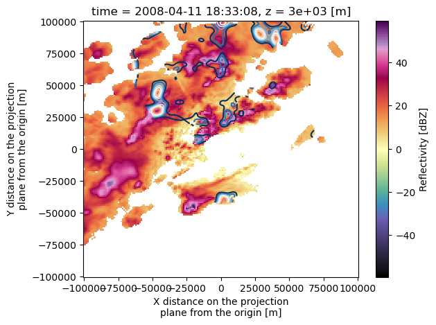
EL (time, z, y, x) float64 -0.5499 -0.5478 ... 5.5ds.reflectivity.sel(z=3000, method='nearest').plot(cmap='pyart_ChaseSpectral')
ds.isel(time=0).sel(z=3000, method='nearest').w.plot.contour(x='x', y='y', levels=np.arange(1, 10, 1))
<matplotlib.contour.QuadContourSet at 0x17dde03d0>
Saving the grids
We can save the grids using either xarray’s or Py-ART’s functionality. To save the output grids, use pyart.io.write_grid (PyART) functions. For example:
pyart.io.write_grid('output_grid_KHTX.nc', grids[0])
pyart.io.write_grid('output_grid_ARMOR.nc', grids[1])
In order to load the grids again, we can just use PyART’s pyart.io.read_grid procedure.
grids = [pyart.io.read_grid('output_grid_KHTX.nc'),
         pyart.io.read_grid('output_grid_ARMOR.nc')]
PyDDA visualization routines
PyDDA’s visualization routines support the native PyART grids that are output by PyDDA. These routines have an advantage over xarray’s plotting routines for adjusting your barb and quiver size by specifying their using parameters that are in scales of kilometers. This makes it easier to plot barb and quiver plots compared to using xarray’s functionality.
For example, the documentation for pydda.vis.plot_horiz_xsection_quiver is given below.
pydda.vis.plot_horiz_xsection_quiver?
Signature:
pydda.vis.plot_horiz_xsection_quiver(
    Grids,
    ax=None,
    background_field='reflectivity',
    level=1,
    cmap='pyart_LangRainbow12',
    vmin=None,
    vmax=None,
    u_vel_contours=None,
    v_vel_contours=None,
    w_vel_contours=None,
    wind_vel_contours=None,
    u_field='u',
    v_field='v',
    w_field='w',
    show_lobes=True,
    title_flag=True,
    axes_labels_flag=True,
    colorbar_flag=True,
    colorbar_contour_flag=False,
    bg_grid_no=0,
    scale=3,
    quiver_spacing_x_km=10.0,
    quiver_spacing_y_km=10.0,
    contour_alpha=0.7,
    quiverkey_len=5.0,
    quiverkey_loc='best',
    quiver_width=0.01,
)
Docstring:
This procedure plots a horizontal cross section of winds from wind fields
generated by PyDDA using quivers. The length of the quivers varies
with horizontal wind speed.

Parameters
----------
Grids: list
    List of Py-ART Grids to visualize
ax: matplotlib axis handle
    The axis handle to place the plot on. Set to None to plot on the
    current axis.
background_field: str
    The name of the background field to plot the quivers on.
level: int
    The number of the vertical level to plot the cross section through.
cmap: str or matplotlib colormap
    The name of the matplotlib colormap to use for the background field.
vmin: float
    The minimum bound to use for plotting the background field. None will
    automatically detect the background field minimum.
vmax: float
    The maximum bound to use for plotting the background field. None will
    automatically detect the background field maximum.
u_vel_contours: 1-D array
    The contours to use for plotting contours of u. Set to None to not
    display such contours.
v_vel_contours: 1-D array
    The contours to use for plotting contours of v. Set to None to not
    display such contours.
w_vel_contours: 1-D array
    The contours to use for plotting contours of w. Set to None to not
    display such contours.
wind_vel_contours: 1-D array
    The contours to use for plotting contours of horizontal wind speed.
    Set to None to not display such contours
u_field: str
    Name of zonal wind (u) field in Grids.
v_field: str
    Name of meridional wind (v) field in Grids.
w_field: str
    Name of vertical wind (w) field in Grids.
show_lobes: bool
    If True, the dual doppler lobes from each pair of radars will be shown.
title_flag: bool
    If True, PyDDA will generate a title for the plot.
axes_labels_flag: bool
    If True, PyDDA will generate axes labels for the plot
colorbar_flag: bool
    If True, PyDDA will generate a colorbar for the plot background field.
colorbar_contour_flag: bool
    If True, PyDDA will generate a colorbar for the contours.
bg_grid_no: int
    Number of grid in Grids to take background field from.
    Set to -1 to use maximum value from all grids.
quiver_spacing_x_km: float
    Spacing in km between quivers in x axis.
quiver_spacing_y_km: float
    Spacing in km between quivers in y axis.
contour_alpha: float
    Alpha (transparency) of velocity contours. 0 = transparent, 1 = opaque
quiverkey_len: float
    Length to use for the quiver key in m/s.
quiverkey_loc: str
    Location of quiverkey. One of:

    'best'

    'top_left'

    'top'

    'top_right'

    'bottom_left'

    'bottom'

    'bottom_right'

    'left'

    'right'

    'top_left_outside'

    'top_right_outside'

    'bottom_left_outside'

    'bottom_right_outside'

    'best' will put the quiver key in the corner with the fewest amount of
     valid data points while keeping the quiver key inside the plot.

     The rest of the options will put the quiver key in that
     particular part of the plot.
quiver_width: float
    The width of the lines for the quiver. Use this to specify
    the thickness of the quiver lines. Units are in fraction of plot
    width.

Returns
-------
ax: Matplotlib axis handle
    The matplotlib axis handle associated with the plot.
File:      ~/PyDDA/pydda/vis/quiver_plot.py
Type:      function
PyDDA has the following visualization routines for your sets of grids:
Procedure |
Description |
|---|---|
plot_horiz_xsection_barbs(Grids[, ax, …]) |
Horizontal cross section of winds from wind fields generated by PyDDA using barbs. |
plot_xz_xsection_barbs(Grids[, ax, …]) |
Cross section of winds from wind fields generated by PyDDA in the X-Z plane using barbs. |
plot_yz_xsection_barbs(Grids[, ax, …]) |
Cross section of winds from wind fields generated by PyDDA in the Y-Z plane using barbs. |
plot_horiz_xsection_barbs_map(Grids[, ax, …]) |
Horizontal cross section of winds from wind fields generated by PyDDA onto a geographical map using barbs. |
plot_horiz_xsection_streamlines(Grids[, ax, …]) |
Horizontal cross section of winds from wind fields generated by PyDDA using streamlines. |
plot_xz_xsection_streamlines(Grids[, ax, …]) |
Cross section of winds from wind fields generated by PyDDA in the X-Z plane using streamlines. |
plot_yz_xsection_streamlines(Grids[, ax, …]) |
Cross section of winds from wind fields generated by PyDDA in the Y-Z plane using streamlines. |
plot_horiz_xsection_streamlines_map(Grids[, …]) |
Horizontal cross section of winds from wind fields generated by PyDDA using streamlines. |
plot_horiz_xsection_quiver(Grids[, ax, …]) |
Horizontal cross section of winds from wind fields generated by PyDDA using quivers. |
plot_xz_xsection_quiver(Grids[, ax, …]) |
Cross section of winds from wind fields generated by PyDDA in the X-Z plane using quivers. |
plot_yz_xsection_quiver(Grids[, ax, …]) |
Cross section of winds from wind fields generated by PyDDA in the Y-Z plane using quivers. |
plot_horiz_xsection_quiver_map(Grids[, ax, …]) |
Horizontal cross section of winds from wind fields generated by PyDDA using quivers onto a geographical map. |
Let’s show a quiver plot of this storm!
We have specified the quivers to be 4 km apart and moved the key to the bottom right with the specific length indicating 20 m/s winds. Let’s look at the 3 km level.
fig, ax = plt.subplots(1, 1, figsize=(6, 6))
pydda.vis.plot_horiz_xsection_quiver(
    grids, quiver_spacing_x_km=10.0, quiver_spacing_y_km=10.0, quiver_width=0.005,
    quiverkey_len=20.0, w_vel_contours=np.arange(2, 15, 1), level=6, cmap='pyart_ChaseSpectral', ax=ax,
    quiverkey_loc='bottom_right')
<AxesSubplot: title={'center': 'PyDDA retreived winds @3.18 km'}, xlabel='X [km]', ylabel='Y [km]'>
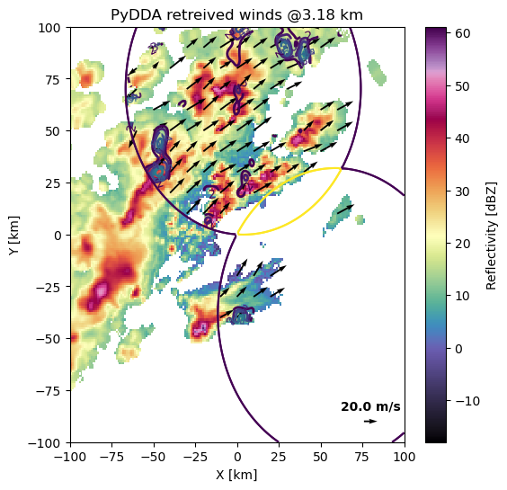
We can zoom in and modify the plot using standard matplotlib functions on the axis handle.
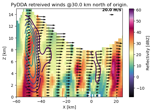
It is much easier to see updrafts being placed just to the outside of the strongest precipitation, with potential new growth in the north of the domain with updraft velocities > 7 m/s. The precipitation is downwind of the updraft as we would expect.
Updrafts are right tilted due to the horizontal wind shear. The horizontal wind shear also causes the most intense precipitation to be downshear of the updraft. This therefore shows us that we have a good quality wind retrieval below about 5 km in altitude.
fig, ax = plt.subplots(1, 1, figsize=(6, 4))
pydda.vis.plot_xz_xsection_quiver(
    grids, quiver_spacing_x_km=8.0, quiver_spacing_z_km=1.0, quiver_width=0.005,
    quiverkey_len=20.0, w_vel_contours=np.arange(2, 20, 2), level=130, cmap='pyart_ChaseSpectral', ax=ax,
    quiverkey_loc='top_right')
ax.set_xlim([-60, 25])
ax.set_ylim([0, 15])
(0.0, 15.0)
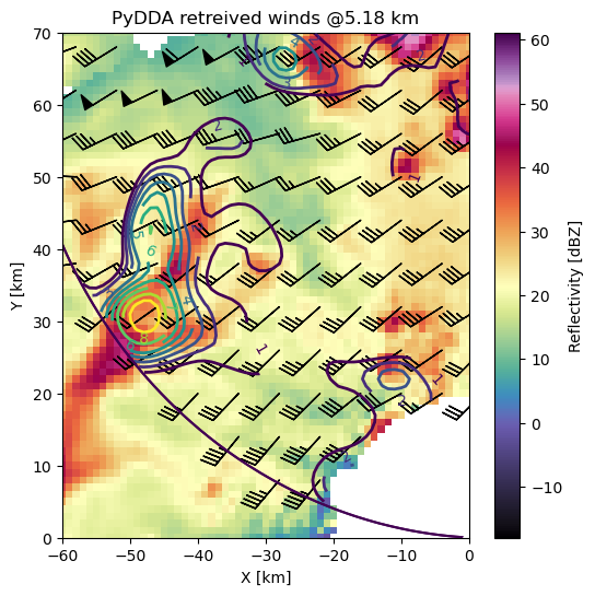
Let’s view a horizontal cross section with barbs!
fig, ax = plt.subplots(1, 1, figsize=(6, 6))
pydda.vis.plot_horiz_xsection_barbs(
    grids, barb_spacing_x_km=6.0, barb_spacing_y_km=6.0,
    w_vel_contours=np.arange(1, 10, 1), level=10, cmap='pyart_ChaseSpectral', ax=ax)
ax.set_xlim([-60, 0])
ax.set_ylim([0, 70])
(0.0, 70.0)