![]()
Xradar Basics
Overview
Within this notebook, we will highlight one of the newer packages in the Open Radar Science ecosystem, Xradar. Here is a brief overview of the motivation of this package:
At a developer meeting held in the course of the ERAD2022 conference in Locarno, Switzerland, future plans and cross-package collaboration of the Open Radar Science community were intensively discussed.

The consensus was that a close collaboration that benefits the entire community can only be maximized through joint projects. So the idea of a common software project whose only task is to read and write radar data was born. The data import should include as many available data formats as possible, but the data export should be limited to the recognized standards, such as ODIM_H5 and CfRadial.

As memory representation an xarray based data model was chosen, which is internally adapted to the forthcoming standard CfRadial2.1/FM301. FM301 is enforced by the Joint Expert Team on Operational Weather Radar (JET-OWR). Information on FM301 is available at WMO as WMO CF Extensions.

Any software package that uses xarray in any way will then be able to directly use the described data model and thus quickly and easily import and export radar data. Another advantage is the easy connection to already existing open source radar processing software.
We will highlight how to get started with xradar, including how to read in data, apply georeferencing, and visualize the datasets.
How to Read in Datasets + Basic Structure
Creating Plan Position Indicator (PPI) Plots Using Georeferencing
Slicing/Dicing Radar Datasets
Prerequisites
Label the importance of each concept explicitly as helpful/necessary.
Concepts |
Importance |
Notes |
|---|---|---|
Required |
Familiarity with Xarray Data Structure |
|
Helpful |
Basic Use of Cartopy Projections |
|
Helpful |
Familiarity with metadata structure |
Time to learn: 15 minutes
Imports
import cmweather
import numpy as np
import xarray as xr
import xradar as xd
import matplotlib.pyplot as plt
import cartopy
How to Read in Datasets + Basic Structure
The first step is reading data. There are two main options here - including
Xarray Backends
Reading Using
xradar.io
Xarray Backends
The first option is to use xarray.backends, where we need to pass which reader to use. Xradar includes the following readers:
cfradial1odimgamicforunorainbowiris(sigmet)
These are passed into the typical xr.open_dataset call, with the reader fed into the engine argument.
For this exercise, we will use data from the University of Alabama Huntsville. They operate a C-band scanning precipitation radar, nicknamed ARMOR. The data from the radar are stored in iris files, a radar data format supported by xradar!
We need to use the iris reader here, specifying which sweep to access. Let’s start with the lowest sweep, sweep_0.
file = "../../data/uah-armor/RAW_NA_000_125_20080411181219"
ds = xr.open_dataset(file,
                     group="sweep_0",
                     engine="iris")
ds
<xarray.Dataset>
Dimensions:            (azimuth: 360, range: 992)
Coordinates:
  * azimuth            (azimuth) float64 0.03296 1.033 1.994 ... 358.0 359.1
    elevation          (azimuth) float32 ...
    time               (azimuth) datetime64[ns] ...
  * range              (range) float32 1e+03 1.125e+03 ... 1.248e+05 1.249e+05
    longitude          float64 ...
    latitude           float64 ...
    altitude           float64 ...
Data variables: (12/13)
    DBTH               (azimuth, range) float32 ...
    DBZH               (azimuth, range) float32 ...
    VRADH              (azimuth, range) float32 ...
    WRADH              (azimuth, range) float32 ...
    ZDR                (azimuth, range) float32 ...
    KDP                (azimuth, range) float32 ...
    ...                 ...
    RHOHV              (azimuth, range) float32 ...
    sweep_mode         <U20 ...
    sweep_number       int64 ...
    prt_mode           <U7 ...
    follow_mode        <U7 ...
sweep_fixed_angle float64 ...- azimuth: 360
- range: 992
- azimuth(azimuth)float640.03296 1.033 1.994 ... 358.0 359.1
- standard_name :
- ray_azimuth_angle
- long_name :
- azimuth_angle_from_true_north
- units :
- degrees
- axis :
- radial_azimuth_coordinate
array([3.295898e-02, 1.032715e+00, 1.994019e+00, ..., 3.569980e+02, 3.580142e+02, 3.590771e+02]) - elevation(azimuth)float32...
- standard_name :
- ray_elevation_angle
- long_name :
- elevation_angle_from_horizontal_plane
- units :
- degrees
- axis :
- radial_elevation_coordinate
[360 values with dtype=float32]
- time(azimuth)datetime64[ns]...
- standard_name :
- time
[360 values with dtype=datetime64[ns]]
- range(range)float321e+03 1.125e+03 ... 1.249e+05
- units :
- meters
- standard_name :
- projection_range_coordinate
- long_name :
- range_to_measurement_volume
- axis :
- radial_range_coordinate
- meters_between_gates :
- 6250.0
- spacing_is_constant :
- true
- meters_to_center_of_first_gate :
- 100000
array([ 1000., 1125., 1250., ..., 124625., 124750., 124875.], dtype=float32) - longitude()float64...
- long_name :
- longitude
- units :
- degrees_east
- standard_name :
- longitude
[1 values with dtype=float64]
- latitude()float64...
- long_name :
- latitude
- units :
- degrees_north
- positive :
- up
- standard_name :
- latitude
[1 values with dtype=float64]
- altitude()float64...
- long_name :
- altitude
- units :
- meters
- standard_name :
- altitude
[1 values with dtype=float64]
- DBTH(azimuth, range)float32...
- units :
- dBZ
- long_name :
- Total power H (uncorrected reflectivity)
- standard_name :
- radar_equivalent_reflectivity_factor_h
- coordinates :
- elevation azimuth range latitude longitude altitude time rtime sweep_mode
[357120 values with dtype=float32]
- DBZH(azimuth, range)float32...
- units :
- dBZ
- long_name :
- Equivalent reflectivity factor H
- standard_name :
- radar_equivalent_reflectivity_factor_h
- coordinates :
- elevation azimuth range latitude longitude altitude time rtime sweep_mode
[357120 values with dtype=float32]
- VRADH(azimuth, range)float32...
- units :
- meters per seconds
- long_name :
- Radial velocity of scatterers away from instrument H
- standard_name :
- radial_velocity_of_scatterers_away_from_instrument_h
- coordinates :
- elevation azimuth range latitude longitude altitude time rtime sweep_mode
[357120 values with dtype=float32]
- WRADH(azimuth, range)float32...
- units :
- meters per seconds
- long_name :
- Doppler spectrum width H
- standard_name :
- radar_doppler_spectrum_width_h
- coordinates :
- elevation azimuth range latitude longitude altitude time rtime sweep_mode
[357120 values with dtype=float32]
- ZDR(azimuth, range)float32...
- units :
- dB
- long_name :
- Log differential reflectivity H/V
- standard_name :
- radar_differential_reflectivity_hv
- coordinates :
- elevation azimuth range latitude longitude altitude time rtime sweep_mode
[357120 values with dtype=float32]
- KDP(azimuth, range)float32...
- units :
- degrees per kilometer
- long_name :
- Specific differential phase HV
- standard_name :
- radar_specific_differential_phase_hv
- coordinates :
- elevation azimuth range latitude longitude altitude time rtime sweep_mode
[357120 values with dtype=float32]
- PHIDP(azimuth, range)float32...
- units :
- degrees
- long_name :
- Differential phase HV
- standard_name :
- radar_differential_phase_hv
- coordinates :
- elevation azimuth range latitude longitude altitude time rtime sweep_mode
[357120 values with dtype=float32]
- RHOHV(azimuth, range)float32...
- units :
- unitless
- long_name :
- Correlation coefficient HV
- standard_name :
- radar_correlation_coefficient_hv
- coordinates :
- elevation azimuth range latitude longitude altitude time rtime sweep_mode
[357120 values with dtype=float32]
- sweep_mode()<U20...
[1 values with dtype=<U20]
- sweep_number()int64...
[1 values with dtype=int64]
- prt_mode()<U7...
[1 values with dtype=<U7]
- follow_mode()<U7...
[1 values with dtype=<U7]
- sweep_fixed_angle()float64...
[1 values with dtype=float64]
- azimuthPandasIndex
PandasIndex(Float64Index([ 0.032958984375, 1.03271484375, 1.9940185546875, 3.06793212890625, 4.04571533203125, 5.0482177734375, 6.0260009765625, 7.064208984375, 8.0364990234375, 9.0472412109375, ... 350.05462646484375, 351.02142333984375, 352.0513916015625, 353.0621337890625, 354.0509033203125, 355.00396728515625, 356.09161376953125, 356.99798583984375, 358.01422119140625, 359.0771484375], dtype='float64', name='azimuth', length=360)) - rangePandasIndex
PandasIndex(Float64Index([  1000.0,   1125.0,   1250.0,   1375.0,   1500.0,   1625.0,
                1750.0,   1875.0,   2000.0,   2125.0,
              ...
              123750.0, 123875.0, 124000.0, 124125.0, 124250.0, 124375.0,
              124500.0, 124625.0, 124750.0, 124875.0],
             dtype='float64', name='range', length=992))
Add a Quick Plot of our Data
Now that we have our xarray.Dataset, we can investigate our data. Let’s start with DBZH, or
Equivalent reflectivity factor H
ds.DBZH.plot(cmap='ChaseSpectral',
             vmin=-32,
             vmax=70)
<matplotlib.collections.QuadMesh at 0x2a30eb040>
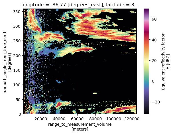
Notice how we have quite a few values of -32 - this is the missing data value for the radar. We can mask this using Xarray!
Reading All of the Sweeps
Let’s read in all of the sweeps from the volume. We need to use the xradar.io.open_iris_datatree
radar = xd.io.open_iris_datatree(file)
radar
<xarray.DatasetView>
Dimensions:              ()
Data variables:
    volume_number        int64 0
    platform_type        <U5 'fixed'
    instrument_type      <U5 'radar'
    time_coverage_start  <U20 '2008-04-11T18:12:20Z'
    time_coverage_end    <U20 '2008-04-11T18:16:17Z'
    longitude            float64 -86.77
    altitude             float64 200.0
    latitude             float64 34.65
Attributes:
    Conventions:      None
    version:          None
    title:            None
    institution:      None
    references:       None
    source:           None
    history:          None
    comment:          im/exported using xradar
instrument_name: None- azimuth: 360
- range: 992
- azimuth(azimuth)float640.03296 1.033 1.994 ... 358.0 359.1
- standard_name :
- ray_azimuth_angle
- long_name :
- azimuth_angle_from_true_north
- units :
- degrees
- axis :
- radial_azimuth_coordinate
array([3.295898e-02, 1.032715e+00, 1.994019e+00, ..., 3.569980e+02, 3.580142e+02, 3.590771e+02]) - elevation(azimuth)float32...
- standard_name :
- ray_elevation_angle
- long_name :
- elevation_angle_from_horizontal_plane
- units :
- degrees
- axis :
- radial_elevation_coordinate
[360 values with dtype=float32]
- time(azimuth)datetime64[ns]2008-04-11T18:12:23.213000 ... 2...
- standard_name :
- time
array(['2008-04-11T18:12:23.213000000', '2008-04-11T18:12:23.213000000', '2008-04-11T18:12:23.213000000', ..., '2008-04-11T18:12:23.213000000', '2008-04-11T18:12:23.213000000', '2008-04-11T18:12:23.213000000'], dtype='datetime64[ns]') - range(range)float321e+03 1.125e+03 ... 1.249e+05
- units :
- meters
- standard_name :
- projection_range_coordinate
- long_name :
- range_to_measurement_volume
- axis :
- radial_range_coordinate
- meters_between_gates :
- 6250.0
- spacing_is_constant :
- true
- meters_to_center_of_first_gate :
- 100000
array([ 1000., 1125., 1250., ..., 124625., 124750., 124875.], dtype=float32) - longitude()float64...
- long_name :
- longitude
- units :
- degrees_east
- standard_name :
- longitude
[1 values with dtype=float64]
- latitude()float64...
- long_name :
- latitude
- units :
- degrees_north
- positive :
- up
- standard_name :
- latitude
[1 values with dtype=float64]
- altitude()float64...
- long_name :
- altitude
- units :
- meters
- standard_name :
- altitude
[1 values with dtype=float64]
- DBTH(azimuth, range)float32...
- units :
- dBZ
- long_name :
- Total power H (uncorrected reflectivity)
- standard_name :
- radar_equivalent_reflectivity_factor_h
- coordinates :
- elevation azimuth range latitude longitude altitude time rtime sweep_mode
[357120 values with dtype=float32]
- DBZH(azimuth, range)float32...
- units :
- dBZ
- long_name :
- Equivalent reflectivity factor H
- standard_name :
- radar_equivalent_reflectivity_factor_h
- coordinates :
- elevation azimuth range latitude longitude altitude time rtime sweep_mode
[357120 values with dtype=float32]
- VRADH(azimuth, range)float32...
- units :
- meters per seconds
- long_name :
- Radial velocity of scatterers away from instrument H
- standard_name :
- radial_velocity_of_scatterers_away_from_instrument_h
- coordinates :
- elevation azimuth range latitude longitude altitude time rtime sweep_mode
[357120 values with dtype=float32]
- WRADH(azimuth, range)float32...
- units :
- meters per seconds
- long_name :
- Doppler spectrum width H
- standard_name :
- radar_doppler_spectrum_width_h
- coordinates :
- elevation azimuth range latitude longitude altitude time rtime sweep_mode
[357120 values with dtype=float32]
- ZDR(azimuth, range)float32...
- units :
- dB
- long_name :
- Log differential reflectivity H/V
- standard_name :
- radar_differential_reflectivity_hv
- coordinates :
- elevation azimuth range latitude longitude altitude time rtime sweep_mode
[357120 values with dtype=float32]
- KDP(azimuth, range)float32...
- units :
- degrees per kilometer
- long_name :
- Specific differential phase HV
- standard_name :
- radar_specific_differential_phase_hv
- coordinates :
- elevation azimuth range latitude longitude altitude time rtime sweep_mode
[357120 values with dtype=float32]
- PHIDP(azimuth, range)float32...
- units :
- degrees
- long_name :
- Differential phase HV
- standard_name :
- radar_differential_phase_hv
- coordinates :
- elevation azimuth range latitude longitude altitude time rtime sweep_mode
[357120 values with dtype=float32]
- RHOHV(azimuth, range)float32...
- units :
- unitless
- long_name :
- Correlation coefficient HV
- standard_name :
- radar_correlation_coefficient_hv
- coordinates :
- elevation azimuth range latitude longitude altitude time rtime sweep_mode
[357120 values with dtype=float32]
- sweep_mode()<U20...
[1 values with dtype=<U20]
- sweep_number()int64...
[1 values with dtype=int64]
- prt_mode()<U7...
[1 values with dtype=<U7]
- follow_mode()<U7...
[1 values with dtype=<U7]
- sweep_fixed_angle()float64...
[1 values with dtype=float64]
<xarray.DatasetView> Dimensions: (azimuth: 360, range: 992) Coordinates: * azimuth (azimuth) float64 0.03296 1.033 1.994 ... 358.0 359.1 elevation (azimuth) float32 ... time (azimuth) datetime64[ns] 2008-04-11T18:12:23.213000 ..... * range (range) float32 1e+03 1.125e+03 ... 1.248e+05 1.249e+05 longitude float64 ... latitude float64 ... altitude float64 ... Data variables: (12/13) DBTH (azimuth, range) float32 ... DBZH (azimuth, range) float32 ... VRADH (azimuth, range) float32 ... WRADH (azimuth, range) float32 ... ZDR (azimuth, range) float32 ... KDP (azimuth, range) float32 ... ... ... RHOHV (azimuth, range) float32 ... sweep_mode <U20 ... sweep_number int64 ... prt_mode <U7 ... follow_mode <U7 ... sweep_fixed_angle float64 ...sweep_0- azimuth: 360
- range: 992
- azimuth(azimuth)float640.07141 1.024 1.991 ... 358.0 359.0
- standard_name :
- ray_azimuth_angle
- long_name :
- azimuth_angle_from_true_north
- units :
- degrees
- axis :
- radial_azimuth_coordinate
array([7.141113e-02, 1.024475e+00, 1.991272e+00, ..., 3.569705e+02, 3.580307e+02, 3.590359e+02]) - elevation(azimuth)float32...
- standard_name :
- ray_elevation_angle
- long_name :
- elevation_angle_from_horizontal_plane
- units :
- degrees
- axis :
- radial_elevation_coordinate
[360 values with dtype=float32]
- time(azimuth)datetime64[ns]2008-04-11T18:12:41.064000 ... 2...
- standard_name :
- time
array(['2008-04-11T18:12:41.064000000', '2008-04-11T18:12:41.064000000', '2008-04-11T18:12:41.064000000', ..., '2008-04-11T18:12:41.064000000', '2008-04-11T18:12:41.064000000', '2008-04-11T18:12:41.064000000'], dtype='datetime64[ns]') - range(range)float321e+03 1.125e+03 ... 1.249e+05
- units :
- meters
- standard_name :
- projection_range_coordinate
- long_name :
- range_to_measurement_volume
- axis :
- radial_range_coordinate
- meters_between_gates :
- 6250.0
- spacing_is_constant :
- true
- meters_to_center_of_first_gate :
- 100000
array([ 1000., 1125., 1250., ..., 124625., 124750., 124875.], dtype=float32) - longitude()float64...
- long_name :
- longitude
- units :
- degrees_east
- standard_name :
- longitude
[1 values with dtype=float64]
- latitude()float64...
- long_name :
- latitude
- units :
- degrees_north
- positive :
- up
- standard_name :
- latitude
[1 values with dtype=float64]
- altitude()float64...
- long_name :
- altitude
- units :
- meters
- standard_name :
- altitude
[1 values with dtype=float64]
- DBTH(azimuth, range)float32...
- units :
- dBZ
- long_name :
- Total power H (uncorrected reflectivity)
- standard_name :
- radar_equivalent_reflectivity_factor_h
- coordinates :
- elevation azimuth range latitude longitude altitude time rtime sweep_mode
[357120 values with dtype=float32]
- DBZH(azimuth, range)float32...
- units :
- dBZ
- long_name :
- Equivalent reflectivity factor H
- standard_name :
- radar_equivalent_reflectivity_factor_h
- coordinates :
- elevation azimuth range latitude longitude altitude time rtime sweep_mode
[357120 values with dtype=float32]
- VRADH(azimuth, range)float32...
- units :
- meters per seconds
- long_name :
- Radial velocity of scatterers away from instrument H
- standard_name :
- radial_velocity_of_scatterers_away_from_instrument_h
- coordinates :
- elevation azimuth range latitude longitude altitude time rtime sweep_mode
[357120 values with dtype=float32]
- WRADH(azimuth, range)float32...
- units :
- meters per seconds
- long_name :
- Doppler spectrum width H
- standard_name :
- radar_doppler_spectrum_width_h
- coordinates :
- elevation azimuth range latitude longitude altitude time rtime sweep_mode
[357120 values with dtype=float32]
- ZDR(azimuth, range)float32...
- units :
- dB
- long_name :
- Log differential reflectivity H/V
- standard_name :
- radar_differential_reflectivity_hv
- coordinates :
- elevation azimuth range latitude longitude altitude time rtime sweep_mode
[357120 values with dtype=float32]
- KDP(azimuth, range)float32...
- units :
- degrees per kilometer
- long_name :
- Specific differential phase HV
- standard_name :
- radar_specific_differential_phase_hv
- coordinates :
- elevation azimuth range latitude longitude altitude time rtime sweep_mode
[357120 values with dtype=float32]
- PHIDP(azimuth, range)float32...
- units :
- degrees
- long_name :
- Differential phase HV
- standard_name :
- radar_differential_phase_hv
- coordinates :
- elevation azimuth range latitude longitude altitude time rtime sweep_mode
[357120 values with dtype=float32]
- RHOHV(azimuth, range)float32...
- units :
- unitless
- long_name :
- Correlation coefficient HV
- standard_name :
- radar_correlation_coefficient_hv
- coordinates :
- elevation azimuth range latitude longitude altitude time rtime sweep_mode
[357120 values with dtype=float32]
- sweep_mode()<U20...
[1 values with dtype=<U20]
- sweep_number()int64...
[1 values with dtype=int64]
- prt_mode()<U7...
[1 values with dtype=<U7]
- follow_mode()<U7...
[1 values with dtype=<U7]
- sweep_fixed_angle()float64...
[1 values with dtype=float64]
<xarray.DatasetView> Dimensions: (azimuth: 360, range: 992) Coordinates: * azimuth (azimuth) float64 0.07141 1.024 1.991 ... 358.0 359.0 elevation (azimuth) float32 ... time (azimuth) datetime64[ns] 2008-04-11T18:12:41.064000 ..... * range (range) float32 1e+03 1.125e+03 ... 1.248e+05 1.249e+05 longitude float64 ... latitude float64 ... altitude float64 ... Data variables: (12/13) DBTH (azimuth, range) float32 ... DBZH (azimuth, range) float32 ... VRADH (azimuth, range) float32 ... WRADH (azimuth, range) float32 ... ZDR (azimuth, range) float32 ... KDP (azimuth, range) float32 ... ... ... RHOHV (azimuth, range) float32 ... sweep_mode <U20 ... sweep_number int64 ... prt_mode <U7 ... follow_mode <U7 ... sweep_fixed_angle float64 ...sweep_1- azimuth: 360
- range: 992
- azimuth(azimuth)float640.06042 1.019 2.019 ... 358.1 359.0
- standard_name :
- ray_azimuth_angle
- long_name :
- azimuth_angle_from_true_north
- units :
- degrees
- axis :
- radial_azimuth_coordinate
array([6.042480e-02, 1.018982e+00, 2.018738e+00, ..., 3.570035e+02, 3.580856e+02, 3.590222e+02]) - elevation(azimuth)float32...
- standard_name :
- ray_elevation_angle
- long_name :
- elevation_angle_from_horizontal_plane
- units :
- degrees
- axis :
- radial_elevation_coordinate
[360 values with dtype=float32]
- time(azimuth)datetime64[ns]2008-04-11T18:13:16.929000 ... 2...
- standard_name :
- time
array(['2008-04-11T18:13:16.929000000', '2008-04-11T18:13:16.929000000', '2008-04-11T18:13:16.929000000', ..., '2008-04-11T18:13:15.929000000', '2008-04-11T18:13:16.929000000', '2008-04-11T18:13:16.929000000'], dtype='datetime64[ns]') - range(range)float321e+03 1.125e+03 ... 1.249e+05
- units :
- meters
- standard_name :
- projection_range_coordinate
- long_name :
- range_to_measurement_volume
- axis :
- radial_range_coordinate
- meters_between_gates :
- 6250.0
- spacing_is_constant :
- true
- meters_to_center_of_first_gate :
- 100000
array([ 1000., 1125., 1250., ..., 124625., 124750., 124875.], dtype=float32) - longitude()float64...
- long_name :
- longitude
- units :
- degrees_east
- standard_name :
- longitude
[1 values with dtype=float64]
- latitude()float64...
- long_name :
- latitude
- units :
- degrees_north
- positive :
- up
- standard_name :
- latitude
[1 values with dtype=float64]
- altitude()float64...
- long_name :
- altitude
- units :
- meters
- standard_name :
- altitude
[1 values with dtype=float64]
- DBTH(azimuth, range)float32...
- units :
- dBZ
- long_name :
- Total power H (uncorrected reflectivity)
- standard_name :
- radar_equivalent_reflectivity_factor_h
- coordinates :
- elevation azimuth range latitude longitude altitude time rtime sweep_mode
[357120 values with dtype=float32]
- DBZH(azimuth, range)float32...
- units :
- dBZ
- long_name :
- Equivalent reflectivity factor H
- standard_name :
- radar_equivalent_reflectivity_factor_h
- coordinates :
- elevation azimuth range latitude longitude altitude time rtime sweep_mode
[357120 values with dtype=float32]
- VRADH(azimuth, range)float32...
- units :
- meters per seconds
- long_name :
- Radial velocity of scatterers away from instrument H
- standard_name :
- radial_velocity_of_scatterers_away_from_instrument_h
- coordinates :
- elevation azimuth range latitude longitude altitude time rtime sweep_mode
[357120 values with dtype=float32]
- WRADH(azimuth, range)float32...
- units :
- meters per seconds
- long_name :
- Doppler spectrum width H
- standard_name :
- radar_doppler_spectrum_width_h
- coordinates :
- elevation azimuth range latitude longitude altitude time rtime sweep_mode
[357120 values with dtype=float32]
- ZDR(azimuth, range)float32...
- units :
- dB
- long_name :
- Log differential reflectivity H/V
- standard_name :
- radar_differential_reflectivity_hv
- coordinates :
- elevation azimuth range latitude longitude altitude time rtime sweep_mode
[357120 values with dtype=float32]
- KDP(azimuth, range)float32...
- units :
- degrees per kilometer
- long_name :
- Specific differential phase HV
- standard_name :
- radar_specific_differential_phase_hv
- coordinates :
- elevation azimuth range latitude longitude altitude time rtime sweep_mode
[357120 values with dtype=float32]
- PHIDP(azimuth, range)float32...
- units :
- degrees
- long_name :
- Differential phase HV
- standard_name :
- radar_differential_phase_hv
- coordinates :
- elevation azimuth range latitude longitude altitude time rtime sweep_mode
[357120 values with dtype=float32]
- RHOHV(azimuth, range)float32...
- units :
- unitless
- long_name :
- Correlation coefficient HV
- standard_name :
- radar_correlation_coefficient_hv
- coordinates :
- elevation azimuth range latitude longitude altitude time rtime sweep_mode
[357120 values with dtype=float32]
- sweep_mode()<U20...
[1 values with dtype=<U20]
- sweep_number()int64...
[1 values with dtype=int64]
- prt_mode()<U7...
[1 values with dtype=<U7]
- follow_mode()<U7...
[1 values with dtype=<U7]
- sweep_fixed_angle()float64...
[1 values with dtype=float64]
<xarray.DatasetView> Dimensions: (azimuth: 360, range: 992) Coordinates: * azimuth (azimuth) float64 0.06042 1.019 2.019 ... 358.1 359.0 elevation (azimuth) float32 ... time (azimuth) datetime64[ns] 2008-04-11T18:13:16.929000 ..... * range (range) float32 1e+03 1.125e+03 ... 1.248e+05 1.249e+05 longitude float64 ... latitude float64 ... altitude float64 ... Data variables: (12/13) DBTH (azimuth, range) float32 ... DBZH (azimuth, range) float32 ... VRADH (azimuth, range) float32 ... WRADH (azimuth, range) float32 ... ZDR (azimuth, range) float32 ... KDP (azimuth, range) float32 ... ... ... RHOHV (azimuth, range) float32 ... sweep_mode <U20 ... sweep_number int64 ... prt_mode <U7 ... follow_mode <U7 ... sweep_fixed_angle float64 ...sweep_2- azimuth: 357
- range: 992
- azimuth(azimuth)float640.03571 1.044 2.021 ... 358.1 359.0
- standard_name :
- ray_azimuth_angle
- long_name :
- azimuth_angle_from_true_north
- units :
- degrees
- axis :
- radial_azimuth_coordinate
array([3.570557e-02, 1.043701e+00, 2.021484e+00, ..., 3.570007e+02, 3.580554e+02, 3.590469e+02]) - elevation(azimuth)float32...
- standard_name :
- ray_elevation_angle
- long_name :
- elevation_angle_from_horizontal_plane
- units :
- degrees
- axis :
- radial_elevation_coordinate
[357 values with dtype=float32]
- time(azimuth)datetime64[ns]2008-04-11T18:13:33.865000 ... 2...
- standard_name :
- time
array(['2008-04-11T18:13:33.865000000', '2008-04-11T18:13:33.865000000', '2008-04-11T18:13:33.865000000', ..., '2008-04-11T18:13:33.865000000', '2008-04-11T18:13:33.865000000', '2008-04-11T18:13:33.865000000'], dtype='datetime64[ns]') - range(range)float321e+03 1.125e+03 ... 1.249e+05
- units :
- meters
- standard_name :
- projection_range_coordinate
- long_name :
- range_to_measurement_volume
- axis :
- radial_range_coordinate
- meters_between_gates :
- 6250.0
- spacing_is_constant :
- true
- meters_to_center_of_first_gate :
- 100000
array([ 1000., 1125., 1250., ..., 124625., 124750., 124875.], dtype=float32) - longitude()float64...
- long_name :
- longitude
- units :
- degrees_east
- standard_name :
- longitude
[1 values with dtype=float64]
- latitude()float64...
- long_name :
- latitude
- units :
- degrees_north
- positive :
- up
- standard_name :
- latitude
[1 values with dtype=float64]
- altitude()float64...
- long_name :
- altitude
- units :
- meters
- standard_name :
- altitude
[1 values with dtype=float64]
- DBTH(azimuth, range)float32...
- units :
- dBZ
- long_name :
- Total power H (uncorrected reflectivity)
- standard_name :
- radar_equivalent_reflectivity_factor_h
- coordinates :
- elevation azimuth range latitude longitude altitude time rtime sweep_mode
[354144 values with dtype=float32]
- DBZH(azimuth, range)float32...
- units :
- dBZ
- long_name :
- Equivalent reflectivity factor H
- standard_name :
- radar_equivalent_reflectivity_factor_h
- coordinates :
- elevation azimuth range latitude longitude altitude time rtime sweep_mode
[354144 values with dtype=float32]
- VRADH(azimuth, range)float32...
- units :
- meters per seconds
- long_name :
- Radial velocity of scatterers away from instrument H
- standard_name :
- radial_velocity_of_scatterers_away_from_instrument_h
- coordinates :
- elevation azimuth range latitude longitude altitude time rtime sweep_mode
[354144 values with dtype=float32]
- WRADH(azimuth, range)float32...
- units :
- meters per seconds
- long_name :
- Doppler spectrum width H
- standard_name :
- radar_doppler_spectrum_width_h
- coordinates :
- elevation azimuth range latitude longitude altitude time rtime sweep_mode
[354144 values with dtype=float32]
- ZDR(azimuth, range)float32...
- units :
- dB
- long_name :
- Log differential reflectivity H/V
- standard_name :
- radar_differential_reflectivity_hv
- coordinates :
- elevation azimuth range latitude longitude altitude time rtime sweep_mode
[354144 values with dtype=float32]
- KDP(azimuth, range)float32...
- units :
- degrees per kilometer
- long_name :
- Specific differential phase HV
- standard_name :
- radar_specific_differential_phase_hv
- coordinates :
- elevation azimuth range latitude longitude altitude time rtime sweep_mode
[354144 values with dtype=float32]
- PHIDP(azimuth, range)float32...
- units :
- degrees
- long_name :
- Differential phase HV
- standard_name :
- radar_differential_phase_hv
- coordinates :
- elevation azimuth range latitude longitude altitude time rtime sweep_mode
[354144 values with dtype=float32]
- RHOHV(azimuth, range)float32...
- units :
- unitless
- long_name :
- Correlation coefficient HV
- standard_name :
- radar_correlation_coefficient_hv
- coordinates :
- elevation azimuth range latitude longitude altitude time rtime sweep_mode
[354144 values with dtype=float32]
- sweep_mode()<U20...
[1 values with dtype=<U20]
- sweep_number()int64...
[1 values with dtype=int64]
- prt_mode()<U7...
[1 values with dtype=<U7]
- follow_mode()<U7...
[1 values with dtype=<U7]
- sweep_fixed_angle()float64...
[1 values with dtype=float64]
<xarray.DatasetView> Dimensions: (azimuth: 357, range: 992) Coordinates: * azimuth (azimuth) float64 0.03571 1.044 2.021 ... 358.1 359.0 elevation (azimuth) float32 ... time (azimuth) datetime64[ns] 2008-04-11T18:13:33.865000 ..... * range (range) float32 1e+03 1.125e+03 ... 1.248e+05 1.249e+05 longitude float64 ... latitude float64 ... altitude float64 ... Data variables: (12/13) DBTH (azimuth, range) float32 ... DBZH (azimuth, range) float32 ... VRADH (azimuth, range) float32 ... WRADH (azimuth, range) float32 ... ZDR (azimuth, range) float32 ... KDP (azimuth, range) float32 ... ... ... RHOHV (azimuth, range) float32 ... sweep_mode <U20 ... sweep_number int64 ... prt_mode <U7 ... follow_mode <U7 ... sweep_fixed_angle float64 ...sweep_3- azimuth: 360
- range: 992
- azimuth(azimuth)float640.06317 0.9915 ... 358.1 359.0
- standard_name :
- ray_azimuth_angle
- long_name :
- azimuth_angle_from_true_north
- units :
- degrees
- axis :
- radial_azimuth_coordinate
array([6.317139e-02, 9.915161e-01, 2.032471e+00, ..., 3.570145e+02, 3.580554e+02, 3.590140e+02]) - elevation(azimuth)float32...
- standard_name :
- ray_elevation_angle
- long_name :
- elevation_angle_from_horizontal_plane
- units :
- degrees
- axis :
- radial_elevation_coordinate
[360 values with dtype=float32]
- time(azimuth)datetime64[ns]2008-04-11T18:13:51.710000 ... 2...
- standard_name :
- time
array(['2008-04-11T18:13:51.710000000', '2008-04-11T18:13:51.710000000', '2008-04-11T18:13:51.710000000', ..., '2008-04-11T18:13:51.710000000', '2008-04-11T18:13:51.710000000', '2008-04-11T18:13:51.710000000'], dtype='datetime64[ns]') - range(range)float321e+03 1.125e+03 ... 1.249e+05
- units :
- meters
- standard_name :
- projection_range_coordinate
- long_name :
- range_to_measurement_volume
- axis :
- radial_range_coordinate
- meters_between_gates :
- 6250.0
- spacing_is_constant :
- true
- meters_to_center_of_first_gate :
- 100000
array([ 1000., 1125., 1250., ..., 124625., 124750., 124875.], dtype=float32) - longitude()float64...
- long_name :
- longitude
- units :
- degrees_east
- standard_name :
- longitude
[1 values with dtype=float64]
- latitude()float64...
- long_name :
- latitude
- units :
- degrees_north
- positive :
- up
- standard_name :
- latitude
[1 values with dtype=float64]
- altitude()float64...
- long_name :
- altitude
- units :
- meters
- standard_name :
- altitude
[1 values with dtype=float64]
- DBTH(azimuth, range)float32...
- units :
- dBZ
- long_name :
- Total power H (uncorrected reflectivity)
- standard_name :
- radar_equivalent_reflectivity_factor_h
- coordinates :
- elevation azimuth range latitude longitude altitude time rtime sweep_mode
[357120 values with dtype=float32]
- DBZH(azimuth, range)float32...
- units :
- dBZ
- long_name :
- Equivalent reflectivity factor H
- standard_name :
- radar_equivalent_reflectivity_factor_h
- coordinates :
- elevation azimuth range latitude longitude altitude time rtime sweep_mode
[357120 values with dtype=float32]
- VRADH(azimuth, range)float32...
- units :
- meters per seconds
- long_name :
- Radial velocity of scatterers away from instrument H
- standard_name :
- radial_velocity_of_scatterers_away_from_instrument_h
- coordinates :
- elevation azimuth range latitude longitude altitude time rtime sweep_mode
[357120 values with dtype=float32]
- WRADH(azimuth, range)float32...
- units :
- meters per seconds
- long_name :
- Doppler spectrum width H
- standard_name :
- radar_doppler_spectrum_width_h
- coordinates :
- elevation azimuth range latitude longitude altitude time rtime sweep_mode
[357120 values with dtype=float32]
- ZDR(azimuth, range)float32...
- units :
- dB
- long_name :
- Log differential reflectivity H/V
- standard_name :
- radar_differential_reflectivity_hv
- coordinates :
- elevation azimuth range latitude longitude altitude time rtime sweep_mode
[357120 values with dtype=float32]
- KDP(azimuth, range)float32...
- units :
- degrees per kilometer
- long_name :
- Specific differential phase HV
- standard_name :
- radar_specific_differential_phase_hv
- coordinates :
- elevation azimuth range latitude longitude altitude time rtime sweep_mode
[357120 values with dtype=float32]
- PHIDP(azimuth, range)float32...
- units :
- degrees
- long_name :
- Differential phase HV
- standard_name :
- radar_differential_phase_hv
- coordinates :
- elevation azimuth range latitude longitude altitude time rtime sweep_mode
[357120 values with dtype=float32]
- RHOHV(azimuth, range)float32...
- units :
- unitless
- long_name :
- Correlation coefficient HV
- standard_name :
- radar_correlation_coefficient_hv
- coordinates :
- elevation azimuth range latitude longitude altitude time rtime sweep_mode
[357120 values with dtype=float32]
- sweep_mode()<U20...
[1 values with dtype=<U20]
- sweep_number()int64...
[1 values with dtype=int64]
- prt_mode()<U7...
[1 values with dtype=<U7]
- follow_mode()<U7...
[1 values with dtype=<U7]
- sweep_fixed_angle()float64...
[1 values with dtype=float64]
<xarray.DatasetView> Dimensions: (azimuth: 360, range: 992) Coordinates: * azimuth (azimuth) float64 0.06317 0.9915 2.032 ... 358.1 359.0 elevation (azimuth) float32 ... time (azimuth) datetime64[ns] 2008-04-11T18:13:51.710000 ..... * range (range) float32 1e+03 1.125e+03 ... 1.248e+05 1.249e+05 longitude float64 ... latitude float64 ... altitude float64 ... Data variables: (12/13) DBTH (azimuth, range) float32 ... DBZH (azimuth, range) float32 ... VRADH (azimuth, range) float32 ... WRADH (azimuth, range) float32 ... ZDR (azimuth, range) float32 ... KDP (azimuth, range) float32 ... ... ... RHOHV (azimuth, range) float32 ... sweep_mode <U20 ... sweep_number int64 ... prt_mode <U7 ... follow_mode <U7 ... sweep_fixed_angle float64 ...sweep_4- azimuth: 359
- range: 992
- azimuth(azimuth)float640.08514 0.9833 2.03 ... 358.0 359.0
- standard_name :
- ray_azimuth_angle
- long_name :
- azimuth_angle_from_true_north
- units :
- degrees
- axis :
- radial_azimuth_coordinate
array([8.514404e-02, 9.832764e-01, 2.029724e+00, ..., 3.569760e+02, 3.580417e+02, 3.590250e+02]) - elevation(azimuth)float32...
- standard_name :
- ray_elevation_angle
- long_name :
- elevation_angle_from_horizontal_plane
- units :
- degrees
- axis :
- radial_elevation_coordinate
[359 values with dtype=float32]
- time(azimuth)datetime64[ns]2008-04-11T18:14:09.747000 ... 2...
- standard_name :
- time
array(['2008-04-11T18:14:09.747000000', '2008-04-11T18:14:09.747000000', '2008-04-11T18:14:09.747000000', ..., '2008-04-11T18:14:09.747000000', '2008-04-11T18:14:09.747000000', '2008-04-11T18:14:09.747000000'], dtype='datetime64[ns]') - range(range)float321e+03 1.125e+03 ... 1.249e+05
- units :
- meters
- standard_name :
- projection_range_coordinate
- long_name :
- range_to_measurement_volume
- axis :
- radial_range_coordinate
- meters_between_gates :
- 6250.0
- spacing_is_constant :
- true
- meters_to_center_of_first_gate :
- 100000
array([ 1000., 1125., 1250., ..., 124625., 124750., 124875.], dtype=float32) - longitude()float64...
- long_name :
- longitude
- units :
- degrees_east
- standard_name :
- longitude
[1 values with dtype=float64]
- latitude()float64...
- long_name :
- latitude
- units :
- degrees_north
- positive :
- up
- standard_name :
- latitude
[1 values with dtype=float64]
- altitude()float64...
- long_name :
- altitude
- units :
- meters
- standard_name :
- altitude
[1 values with dtype=float64]
- DBTH(azimuth, range)float32...
- units :
- dBZ
- long_name :
- Total power H (uncorrected reflectivity)
- standard_name :
- radar_equivalent_reflectivity_factor_h
- coordinates :
- elevation azimuth range latitude longitude altitude time rtime sweep_mode
[356128 values with dtype=float32]
- DBZH(azimuth, range)float32...
- units :
- dBZ
- long_name :
- Equivalent reflectivity factor H
- standard_name :
- radar_equivalent_reflectivity_factor_h
- coordinates :
- elevation azimuth range latitude longitude altitude time rtime sweep_mode
[356128 values with dtype=float32]
- VRADH(azimuth, range)float32...
- units :
- meters per seconds
- long_name :
- Radial velocity of scatterers away from instrument H
- standard_name :
- radial_velocity_of_scatterers_away_from_instrument_h
- coordinates :
- elevation azimuth range latitude longitude altitude time rtime sweep_mode
[356128 values with dtype=float32]
- WRADH(azimuth, range)float32...
- units :
- meters per seconds
- long_name :
- Doppler spectrum width H
- standard_name :
- radar_doppler_spectrum_width_h
- coordinates :
- elevation azimuth range latitude longitude altitude time rtime sweep_mode
[356128 values with dtype=float32]
- ZDR(azimuth, range)float32...
- units :
- dB
- long_name :
- Log differential reflectivity H/V
- standard_name :
- radar_differential_reflectivity_hv
- coordinates :
- elevation azimuth range latitude longitude altitude time rtime sweep_mode
[356128 values with dtype=float32]
- KDP(azimuth, range)float32...
- units :
- degrees per kilometer
- long_name :
- Specific differential phase HV
- standard_name :
- radar_specific_differential_phase_hv
- coordinates :
- elevation azimuth range latitude longitude altitude time rtime sweep_mode
[356128 values with dtype=float32]
- PHIDP(azimuth, range)float32...
- units :
- degrees
- long_name :
- Differential phase HV
- standard_name :
- radar_differential_phase_hv
- coordinates :
- elevation azimuth range latitude longitude altitude time rtime sweep_mode
[356128 values with dtype=float32]
- RHOHV(azimuth, range)float32...
- units :
- unitless
- long_name :
- Correlation coefficient HV
- standard_name :
- radar_correlation_coefficient_hv
- coordinates :
- elevation azimuth range latitude longitude altitude time rtime sweep_mode
[356128 values with dtype=float32]
- sweep_mode()<U20...
[1 values with dtype=<U20]
- sweep_number()int64...
[1 values with dtype=int64]
- prt_mode()<U7...
[1 values with dtype=<U7]
- follow_mode()<U7...
[1 values with dtype=<U7]
- sweep_fixed_angle()float64...
[1 values with dtype=float64]
<xarray.DatasetView> Dimensions: (azimuth: 359, range: 992) Coordinates: * azimuth (azimuth) float64 0.08514 0.9833 2.03 ... 358.0 359.0 elevation (azimuth) float32 ... time (azimuth) datetime64[ns] 2008-04-11T18:14:09.747000 ..... * range (range) float32 1e+03 1.125e+03 ... 1.248e+05 1.249e+05 longitude float64 ... latitude float64 ... altitude float64 ... Data variables: (12/13) DBTH (azimuth, range) float32 ... DBZH (azimuth, range) float32 ... VRADH (azimuth, range) float32 ... WRADH (azimuth, range) float32 ... ZDR (azimuth, range) float32 ... KDP (azimuth, range) float32 ... ... ... RHOHV (azimuth, range) float32 ... sweep_mode <U20 ... sweep_number int64 ... prt_mode <U7 ... follow_mode <U7 ... sweep_fixed_angle float64 ...sweep_5- azimuth: 360
- range: 992
- azimuth(azimuth)float640.05219 1.115 1.983 ... 358.0 359.0
- standard_name :
- ray_azimuth_angle
- long_name :
- azimuth_angle_from_true_north
- units :
- degrees
- axis :
- radial_azimuth_coordinate
array([5.218506e-02, 1.115112e+00, 1.983032e+00, ..., 3.570255e+02, 3.580389e+02, 3.590497e+02]) - elevation(azimuth)float32...
- standard_name :
- ray_elevation_angle
- long_name :
- elevation_angle_from_horizontal_plane
- units :
- degrees
- axis :
- radial_elevation_coordinate
[360 values with dtype=float32]
- time(azimuth)datetime64[ns]2008-04-11T18:14:27.735000 ... 2...
- standard_name :
- time
array(['2008-04-11T18:14:27.735000000', '2008-04-11T18:14:27.735000000', '2008-04-11T18:14:27.735000000', ..., '2008-04-11T18:14:26.735000000', '2008-04-11T18:14:26.735000000', '2008-04-11T18:14:27.735000000'], dtype='datetime64[ns]') - range(range)float321e+03 1.125e+03 ... 1.249e+05
- units :
- meters
- standard_name :
- projection_range_coordinate
- long_name :
- range_to_measurement_volume
- axis :
- radial_range_coordinate
- meters_between_gates :
- 6250.0
- spacing_is_constant :
- true
- meters_to_center_of_first_gate :
- 100000
array([ 1000., 1125., 1250., ..., 124625., 124750., 124875.], dtype=float32) - longitude()float64...
- long_name :
- longitude
- units :
- degrees_east
- standard_name :
- longitude
[1 values with dtype=float64]
- latitude()float64...
- long_name :
- latitude
- units :
- degrees_north
- positive :
- up
- standard_name :
- latitude
[1 values with dtype=float64]
- altitude()float64...
- long_name :
- altitude
- units :
- meters
- standard_name :
- altitude
[1 values with dtype=float64]
- DBTH(azimuth, range)float32...
- units :
- dBZ
- long_name :
- Total power H (uncorrected reflectivity)
- standard_name :
- radar_equivalent_reflectivity_factor_h
- coordinates :
- elevation azimuth range latitude longitude altitude time rtime sweep_mode
[357120 values with dtype=float32]
- DBZH(azimuth, range)float32...
- units :
- dBZ
- long_name :
- Equivalent reflectivity factor H
- standard_name :
- radar_equivalent_reflectivity_factor_h
- coordinates :
- elevation azimuth range latitude longitude altitude time rtime sweep_mode
[357120 values with dtype=float32]
- VRADH(azimuth, range)float32...
- units :
- meters per seconds
- long_name :
- Radial velocity of scatterers away from instrument H
- standard_name :
- radial_velocity_of_scatterers_away_from_instrument_h
- coordinates :
- elevation azimuth range latitude longitude altitude time rtime sweep_mode
[357120 values with dtype=float32]
- WRADH(azimuth, range)float32...
- units :
- meters per seconds
- long_name :
- Doppler spectrum width H
- standard_name :
- radar_doppler_spectrum_width_h
- coordinates :
- elevation azimuth range latitude longitude altitude time rtime sweep_mode
[357120 values with dtype=float32]
- ZDR(azimuth, range)float32...
- units :
- dB
- long_name :
- Log differential reflectivity H/V
- standard_name :
- radar_differential_reflectivity_hv
- coordinates :
- elevation azimuth range latitude longitude altitude time rtime sweep_mode
[357120 values with dtype=float32]
- KDP(azimuth, range)float32...
- units :
- degrees per kilometer
- long_name :
- Specific differential phase HV
- standard_name :
- radar_specific_differential_phase_hv
- coordinates :
- elevation azimuth range latitude longitude altitude time rtime sweep_mode
[357120 values with dtype=float32]
- PHIDP(azimuth, range)float32...
- units :
- degrees
- long_name :
- Differential phase HV
- standard_name :
- radar_differential_phase_hv
- coordinates :
- elevation azimuth range latitude longitude altitude time rtime sweep_mode
[357120 values with dtype=float32]
- RHOHV(azimuth, range)float32...
- units :
- unitless
- long_name :
- Correlation coefficient HV
- standard_name :
- radar_correlation_coefficient_hv
- coordinates :
- elevation azimuth range latitude longitude altitude time rtime sweep_mode
[357120 values with dtype=float32]
- sweep_mode()<U20...
[1 values with dtype=<U20]
- sweep_number()int64...
[1 values with dtype=int64]
- prt_mode()<U7...
[1 values with dtype=<U7]
- follow_mode()<U7...
[1 values with dtype=<U7]
- sweep_fixed_angle()float64...
[1 values with dtype=float64]
<xarray.DatasetView> Dimensions: (azimuth: 360, range: 992) Coordinates: * azimuth (azimuth) float64 0.05219 1.115 1.983 ... 358.0 359.0 elevation (azimuth) float32 ... time (azimuth) datetime64[ns] 2008-04-11T18:14:27.735000 ..... * range (range) float32 1e+03 1.125e+03 ... 1.248e+05 1.249e+05 longitude float64 ... latitude float64 ... altitude float64 ... Data variables: (12/13) DBTH (azimuth, range) float32 ... DBZH (azimuth, range) float32 ... VRADH (azimuth, range) float32 ... WRADH (azimuth, range) float32 ... ZDR (azimuth, range) float32 ... KDP (azimuth, range) float32 ... ... ... RHOHV (azimuth, range) float32 ... sweep_mode <U20 ... sweep_number int64 ... prt_mode <U7 ... follow_mode <U7 ... sweep_fixed_angle float64 ...sweep_6- azimuth: 358
- range: 992
- azimuth(azimuth)float640.04944 1.003 2.032 ... 358.1 359.0
- standard_name :
- ray_azimuth_angle
- long_name :
- azimuth_angle_from_true_north
- units :
- degrees
- axis :
- radial_azimuth_coordinate
array([4.943848e-02, 1.002502e+00, 2.032471e+00, ..., 3.569733e+02, 3.581186e+02, 3.590387e+02]) - elevation(azimuth)float32...
- standard_name :
- ray_elevation_angle
- long_name :
- elevation_angle_from_horizontal_plane
- units :
- degrees
- axis :
- radial_elevation_coordinate
[358 values with dtype=float32]
- time(azimuth)datetime64[ns]2008-04-11T18:14:44.727000 ... 2...
- standard_name :
- time
array(['2008-04-11T18:14:44.727000000', '2008-04-11T18:14:44.727000000', '2008-04-11T18:14:44.727000000', ..., '2008-04-11T18:14:44.727000000', '2008-04-11T18:14:44.727000000', '2008-04-11T18:14:44.727000000'], dtype='datetime64[ns]') - range(range)float321e+03 1.125e+03 ... 1.249e+05
- units :
- meters
- standard_name :
- projection_range_coordinate
- long_name :
- range_to_measurement_volume
- axis :
- radial_range_coordinate
- meters_between_gates :
- 6250.0
- spacing_is_constant :
- true
- meters_to_center_of_first_gate :
- 100000
array([ 1000., 1125., 1250., ..., 124625., 124750., 124875.], dtype=float32) - longitude()float64...
- long_name :
- longitude
- units :
- degrees_east
- standard_name :
- longitude
[1 values with dtype=float64]
- latitude()float64...
- long_name :
- latitude
- units :
- degrees_north
- positive :
- up
- standard_name :
- latitude
[1 values with dtype=float64]
- altitude()float64...
- long_name :
- altitude
- units :
- meters
- standard_name :
- altitude
[1 values with dtype=float64]
- DBTH(azimuth, range)float32...
- units :
- dBZ
- long_name :
- Total power H (uncorrected reflectivity)
- standard_name :
- radar_equivalent_reflectivity_factor_h
- coordinates :
- elevation azimuth range latitude longitude altitude time rtime sweep_mode
[355136 values with dtype=float32]
- DBZH(azimuth, range)float32...
- units :
- dBZ
- long_name :
- Equivalent reflectivity factor H
- standard_name :
- radar_equivalent_reflectivity_factor_h
- coordinates :
- elevation azimuth range latitude longitude altitude time rtime sweep_mode
[355136 values with dtype=float32]
- VRADH(azimuth, range)float32...
- units :
- meters per seconds
- long_name :
- Radial velocity of scatterers away from instrument H
- standard_name :
- radial_velocity_of_scatterers_away_from_instrument_h
- coordinates :
- elevation azimuth range latitude longitude altitude time rtime sweep_mode
[355136 values with dtype=float32]
- WRADH(azimuth, range)float32...
- units :
- meters per seconds
- long_name :
- Doppler spectrum width H
- standard_name :
- radar_doppler_spectrum_width_h
- coordinates :
- elevation azimuth range latitude longitude altitude time rtime sweep_mode
[355136 values with dtype=float32]
- ZDR(azimuth, range)float32...
- units :
- dB
- long_name :
- Log differential reflectivity H/V
- standard_name :
- radar_differential_reflectivity_hv
- coordinates :
- elevation azimuth range latitude longitude altitude time rtime sweep_mode
[355136 values with dtype=float32]
- KDP(azimuth, range)float32...
- units :
- degrees per kilometer
- long_name :
- Specific differential phase HV
- standard_name :
- radar_specific_differential_phase_hv
- coordinates :
- elevation azimuth range latitude longitude altitude time rtime sweep_mode
[355136 values with dtype=float32]
- PHIDP(azimuth, range)float32...
- units :
- degrees
- long_name :
- Differential phase HV
- standard_name :
- radar_differential_phase_hv
- coordinates :
- elevation azimuth range latitude longitude altitude time rtime sweep_mode
[355136 values with dtype=float32]
- RHOHV(azimuth, range)float32...
- units :
- unitless
- long_name :
- Correlation coefficient HV
- standard_name :
- radar_correlation_coefficient_hv
- coordinates :
- elevation azimuth range latitude longitude altitude time rtime sweep_mode
[355136 values with dtype=float32]
- sweep_mode()<U20...
[1 values with dtype=<U20]
- sweep_number()int64...
[1 values with dtype=int64]
- prt_mode()<U7...
[1 values with dtype=<U7]
- follow_mode()<U7...
[1 values with dtype=<U7]
- sweep_fixed_angle()float64...
[1 values with dtype=float64]
<xarray.DatasetView> Dimensions: (azimuth: 358, range: 992) Coordinates: * azimuth (azimuth) float64 0.04944 1.003 2.032 ... 358.1 359.0 elevation (azimuth) float32 ... time (azimuth) datetime64[ns] 2008-04-11T18:14:44.727000 ..... * range (range) float32 1e+03 1.125e+03 ... 1.248e+05 1.249e+05 longitude float64 ... latitude float64 ... altitude float64 ... Data variables: (12/13) DBTH (azimuth, range) float32 ... DBZH (azimuth, range) float32 ... VRADH (azimuth, range) float32 ... WRADH (azimuth, range) float32 ... ZDR (azimuth, range) float32 ... KDP (azimuth, range) float32 ... ... ... RHOHV (azimuth, range) float32 ... sweep_mode <U20 ... sweep_number int64 ... prt_mode <U7 ... follow_mode <U7 ... sweep_fixed_angle float64 ...sweep_7- azimuth: 360
- range: 992
- azimuth(azimuth)float640.05219 1.019 2.008 ... 358.0 359.0
- standard_name :
- ray_azimuth_angle
- long_name :
- azimuth_angle_from_true_north
- units :
- degrees
- axis :
- radial_azimuth_coordinate
array([5.218506e-02, 1.018982e+00, 2.007751e+00, ..., 3.570694e+02, 3.579703e+02, 3.590305e+02]) - elevation(azimuth)float32...
- standard_name :
- ray_elevation_angle
- long_name :
- elevation_angle_from_horizontal_plane
- units :
- degrees
- axis :
- radial_elevation_coordinate
[360 values with dtype=float32]
- time(azimuth)datetime64[ns]2008-04-11T18:15:02.728000 ... 2...
- standard_name :
- time
array(['2008-04-11T18:15:02.728000000', '2008-04-11T18:15:02.728000000', '2008-04-11T18:15:02.728000000', ..., '2008-04-11T18:15:02.728000000', '2008-04-11T18:15:02.728000000', '2008-04-11T18:15:02.728000000'], dtype='datetime64[ns]') - range(range)float321e+03 1.125e+03 ... 1.249e+05
- units :
- meters
- standard_name :
- projection_range_coordinate
- long_name :
- range_to_measurement_volume
- axis :
- radial_range_coordinate
- meters_between_gates :
- 6250.0
- spacing_is_constant :
- true
- meters_to_center_of_first_gate :
- 100000
array([ 1000., 1125., 1250., ..., 124625., 124750., 124875.], dtype=float32) - longitude()float64...
- long_name :
- longitude
- units :
- degrees_east
- standard_name :
- longitude
[1 values with dtype=float64]
- latitude()float64...
- long_name :
- latitude
- units :
- degrees_north
- positive :
- up
- standard_name :
- latitude
[1 values with dtype=float64]
- altitude()float64...
- long_name :
- altitude
- units :
- meters
- standard_name :
- altitude
[1 values with dtype=float64]
- DBTH(azimuth, range)float32...
- units :
- dBZ
- long_name :
- Total power H (uncorrected reflectivity)
- standard_name :
- radar_equivalent_reflectivity_factor_h
- coordinates :
- elevation azimuth range latitude longitude altitude time rtime sweep_mode
[357120 values with dtype=float32]
- DBZH(azimuth, range)float32...
- units :
- dBZ
- long_name :
- Equivalent reflectivity factor H
- standard_name :
- radar_equivalent_reflectivity_factor_h
- coordinates :
- elevation azimuth range latitude longitude altitude time rtime sweep_mode
[357120 values with dtype=float32]
- VRADH(azimuth, range)float32...
- units :
- meters per seconds
- long_name :
- Radial velocity of scatterers away from instrument H
- standard_name :
- radial_velocity_of_scatterers_away_from_instrument_h
- coordinates :
- elevation azimuth range latitude longitude altitude time rtime sweep_mode
[357120 values with dtype=float32]
- WRADH(azimuth, range)float32...
- units :
- meters per seconds
- long_name :
- Doppler spectrum width H
- standard_name :
- radar_doppler_spectrum_width_h
- coordinates :
- elevation azimuth range latitude longitude altitude time rtime sweep_mode
[357120 values with dtype=float32]
- ZDR(azimuth, range)float32...
- units :
- dB
- long_name :
- Log differential reflectivity H/V
- standard_name :
- radar_differential_reflectivity_hv
- coordinates :
- elevation azimuth range latitude longitude altitude time rtime sweep_mode
[357120 values with dtype=float32]
- KDP(azimuth, range)float32...
- units :
- degrees per kilometer
- long_name :
- Specific differential phase HV
- standard_name :
- radar_specific_differential_phase_hv
- coordinates :
- elevation azimuth range latitude longitude altitude time rtime sweep_mode
[357120 values with dtype=float32]
- PHIDP(azimuth, range)float32...
- units :
- degrees
- long_name :
- Differential phase HV
- standard_name :
- radar_differential_phase_hv
- coordinates :
- elevation azimuth range latitude longitude altitude time rtime sweep_mode
[357120 values with dtype=float32]
- RHOHV(azimuth, range)float32...
- units :
- unitless
- long_name :
- Correlation coefficient HV
- standard_name :
- radar_correlation_coefficient_hv
- coordinates :
- elevation azimuth range latitude longitude altitude time rtime sweep_mode
[357120 values with dtype=float32]
- sweep_mode()<U20...
[1 values with dtype=<U20]
- sweep_number()int64...
[1 values with dtype=int64]
- prt_mode()<U7...
[1 values with dtype=<U7]
- follow_mode()<U7...
[1 values with dtype=<U7]
- sweep_fixed_angle()float64...
[1 values with dtype=float64]
<xarray.DatasetView> Dimensions: (azimuth: 360, range: 992) Coordinates: * azimuth (azimuth) float64 0.05219 1.019 2.008 ... 358.0 359.0 elevation (azimuth) float32 ... time (azimuth) datetime64[ns] 2008-04-11T18:15:02.728000 ..... * range (range) float32 1e+03 1.125e+03 ... 1.248e+05 1.249e+05 longitude float64 ... latitude float64 ... altitude float64 ... Data variables: (12/13) DBTH (azimuth, range) float32 ... DBZH (azimuth, range) float32 ... VRADH (azimuth, range) float32 ... WRADH (azimuth, range) float32 ... ZDR (azimuth, range) float32 ... KDP (azimuth, range) float32 ... ... ... RHOHV (azimuth, range) float32 ... sweep_mode <U20 ... sweep_number int64 ... prt_mode <U7 ... follow_mode <U7 ... sweep_fixed_angle float64 ...sweep_8- azimuth: 360
- range: 992
- azimuth(azimuth)float641.046 2.038 3.049 ... 359.0 360.0
- standard_name :
- ray_azimuth_angle
- long_name :
- azimuth_angle_from_true_north
- units :
- degrees
- axis :
- radial_azimuth_coordinate
array([ 1.046448, 2.037964, 3.048706, ..., 358.06366 , 359.049683, 359.983521]) - elevation(azimuth)float32...
- standard_name :
- ray_elevation_angle
- long_name :
- elevation_angle_from_horizontal_plane
- units :
- degrees
- axis :
- radial_elevation_coordinate
[360 values with dtype=float32]
- time(azimuth)datetime64[ns]2008-04-11T18:15:37.925000 ... 2...
- standard_name :
- time
array(['2008-04-11T18:15:37.925000000', '2008-04-11T18:15:37.925000000', '2008-04-11T18:15:20.925000000', ..., '2008-04-11T18:15:37.925000000', '2008-04-11T18:15:37.925000000', '2008-04-11T18:15:37.925000000'], dtype='datetime64[ns]') - range(range)float321e+03 1.125e+03 ... 1.249e+05
- units :
- meters
- standard_name :
- projection_range_coordinate
- long_name :
- range_to_measurement_volume
- axis :
- radial_range_coordinate
- meters_between_gates :
- 6250.0
- spacing_is_constant :
- true
- meters_to_center_of_first_gate :
- 100000
array([ 1000., 1125., 1250., ..., 124625., 124750., 124875.], dtype=float32) - longitude()float64...
- long_name :
- longitude
- units :
- degrees_east
- standard_name :
- longitude
[1 values with dtype=float64]
- latitude()float64...
- long_name :
- latitude
- units :
- degrees_north
- positive :
- up
- standard_name :
- latitude
[1 values with dtype=float64]
- altitude()float64...
- long_name :
- altitude
- units :
- meters
- standard_name :
- altitude
[1 values with dtype=float64]
- DBTH(azimuth, range)float32...
- units :
- dBZ
- long_name :
- Total power H (uncorrected reflectivity)
- standard_name :
- radar_equivalent_reflectivity_factor_h
- coordinates :
- elevation azimuth range latitude longitude altitude time rtime sweep_mode
[357120 values with dtype=float32]
- DBZH(azimuth, range)float32...
- units :
- dBZ
- long_name :
- Equivalent reflectivity factor H
- standard_name :
- radar_equivalent_reflectivity_factor_h
- coordinates :
- elevation azimuth range latitude longitude altitude time rtime sweep_mode
[357120 values with dtype=float32]
- VRADH(azimuth, range)float32...
- units :
- meters per seconds
- long_name :
- Radial velocity of scatterers away from instrument H
- standard_name :
- radial_velocity_of_scatterers_away_from_instrument_h
- coordinates :
- elevation azimuth range latitude longitude altitude time rtime sweep_mode
[357120 values with dtype=float32]
- WRADH(azimuth, range)float32...
- units :
- meters per seconds
- long_name :
- Doppler spectrum width H
- standard_name :
- radar_doppler_spectrum_width_h
- coordinates :
- elevation azimuth range latitude longitude altitude time rtime sweep_mode
[357120 values with dtype=float32]
- ZDR(azimuth, range)float32...
- units :
- dB
- long_name :
- Log differential reflectivity H/V
- standard_name :
- radar_differential_reflectivity_hv
- coordinates :
- elevation azimuth range latitude longitude altitude time rtime sweep_mode
[357120 values with dtype=float32]
- KDP(azimuth, range)float32...
- units :
- degrees per kilometer
- long_name :
- Specific differential phase HV
- standard_name :
- radar_specific_differential_phase_hv
- coordinates :
- elevation azimuth range latitude longitude altitude time rtime sweep_mode
[357120 values with dtype=float32]
- PHIDP(azimuth, range)float32...
- units :
- degrees
- long_name :
- Differential phase HV
- standard_name :
- radar_differential_phase_hv
- coordinates :
- elevation azimuth range latitude longitude altitude time rtime sweep_mode
[357120 values with dtype=float32]
- RHOHV(azimuth, range)float32...
- units :
- unitless
- long_name :
- Correlation coefficient HV
- standard_name :
- radar_correlation_coefficient_hv
- coordinates :
- elevation azimuth range latitude longitude altitude time rtime sweep_mode
[357120 values with dtype=float32]
- sweep_mode()<U20...
[1 values with dtype=<U20]
- sweep_number()int64...
[1 values with dtype=int64]
- prt_mode()<U7...
[1 values with dtype=<U7]
- follow_mode()<U7...
[1 values with dtype=<U7]
- sweep_fixed_angle()float64...
[1 values with dtype=float64]
<xarray.DatasetView> Dimensions: (azimuth: 360, range: 992) Coordinates: * azimuth (azimuth) float64 1.046 2.038 3.049 ... 358.1 359.0 360.0 elevation (azimuth) float32 ... time (azimuth) datetime64[ns] 2008-04-11T18:15:37.925000 ..... * range (range) float32 1e+03 1.125e+03 ... 1.248e+05 1.249e+05 longitude float64 ... latitude float64 ... altitude float64 ... Data variables: (12/13) DBTH (azimuth, range) float32 ... DBZH (azimuth, range) float32 ... VRADH (azimuth, range) float32 ... WRADH (azimuth, range) float32 ... ZDR (azimuth, range) float32 ... KDP (azimuth, range) float32 ... ... ... RHOHV (azimuth, range) float32 ... sweep_mode <U20 ... sweep_number int64 ... prt_mode <U7 ... follow_mode <U7 ... sweep_fixed_angle float64 ...sweep_9- azimuth: 360
- range: 992
- azimuth(azimuth)float640.0412 1.049 2.0 ... 358.0 359.0
- standard_name :
- ray_azimuth_angle
- long_name :
- azimuth_angle_from_true_north
- units :
- degrees
- axis :
- radial_azimuth_coordinate
array([4.119873e-02, 1.049194e+00, 1.999512e+00, ..., 3.571188e+02, 3.579950e+02, 3.590140e+02]) - elevation(azimuth)float32...
- standard_name :
- ray_elevation_angle
- long_name :
- elevation_angle_from_horizontal_plane
- units :
- degrees
- axis :
- radial_elevation_coordinate
[360 values with dtype=float32]
- time(azimuth)datetime64[ns]2008-04-11T18:15:56.106000 ... 2...
- standard_name :
- time
array(['2008-04-11T18:15:56.106000000', '2008-04-11T18:15:56.106000000', '2008-04-11T18:15:56.106000000', ..., '2008-04-11T18:15:55.106000000', '2008-04-11T18:15:56.106000000', '2008-04-11T18:15:56.106000000'], dtype='datetime64[ns]') - range(range)float321e+03 1.125e+03 ... 1.249e+05
- units :
- meters
- standard_name :
- projection_range_coordinate
- long_name :
- range_to_measurement_volume
- axis :
- radial_range_coordinate
- meters_between_gates :
- 6250.0
- spacing_is_constant :
- true
- meters_to_center_of_first_gate :
- 100000
array([ 1000., 1125., 1250., ..., 124625., 124750., 124875.], dtype=float32) - longitude()float64...
- long_name :
- longitude
- units :
- degrees_east
- standard_name :
- longitude
[1 values with dtype=float64]
- latitude()float64...
- long_name :
- latitude
- units :
- degrees_north
- positive :
- up
- standard_name :
- latitude
[1 values with dtype=float64]
- altitude()float64...
- long_name :
- altitude
- units :
- meters
- standard_name :
- altitude
[1 values with dtype=float64]
- DBTH(azimuth, range)float32...
- units :
- dBZ
- long_name :
- Total power H (uncorrected reflectivity)
- standard_name :
- radar_equivalent_reflectivity_factor_h
- coordinates :
- elevation azimuth range latitude longitude altitude time rtime sweep_mode
[357120 values with dtype=float32]
- DBZH(azimuth, range)float32...
- units :
- dBZ
- long_name :
- Equivalent reflectivity factor H
- standard_name :
- radar_equivalent_reflectivity_factor_h
- coordinates :
- elevation azimuth range latitude longitude altitude time rtime sweep_mode
[357120 values with dtype=float32]
- VRADH(azimuth, range)float32...
- units :
- meters per seconds
- long_name :
- Radial velocity of scatterers away from instrument H
- standard_name :
- radial_velocity_of_scatterers_away_from_instrument_h
- coordinates :
- elevation azimuth range latitude longitude altitude time rtime sweep_mode
[357120 values with dtype=float32]
- WRADH(azimuth, range)float32...
- units :
- meters per seconds
- long_name :
- Doppler spectrum width H
- standard_name :
- radar_doppler_spectrum_width_h
- coordinates :
- elevation azimuth range latitude longitude altitude time rtime sweep_mode
[357120 values with dtype=float32]
- ZDR(azimuth, range)float32...
- units :
- dB
- long_name :
- Log differential reflectivity H/V
- standard_name :
- radar_differential_reflectivity_hv
- coordinates :
- elevation azimuth range latitude longitude altitude time rtime sweep_mode
[357120 values with dtype=float32]
- KDP(azimuth, range)float32...
- units :
- degrees per kilometer
- long_name :
- Specific differential phase HV
- standard_name :
- radar_specific_differential_phase_hv
- coordinates :
- elevation azimuth range latitude longitude altitude time rtime sweep_mode
[357120 values with dtype=float32]
- PHIDP(azimuth, range)float32...
- units :
- degrees
- long_name :
- Differential phase HV
- standard_name :
- radar_differential_phase_hv
- coordinates :
- elevation azimuth range latitude longitude altitude time rtime sweep_mode
[357120 values with dtype=float32]
- RHOHV(azimuth, range)float32...
- units :
- unitless
- long_name :
- Correlation coefficient HV
- standard_name :
- radar_correlation_coefficient_hv
- coordinates :
- elevation azimuth range latitude longitude altitude time rtime sweep_mode
[357120 values with dtype=float32]
- sweep_mode()<U20...
[1 values with dtype=<U20]
- sweep_number()int64...
[1 values with dtype=int64]
- prt_mode()<U7...
[1 values with dtype=<U7]
- follow_mode()<U7...
[1 values with dtype=<U7]
- sweep_fixed_angle()float64...
[1 values with dtype=float64]
<xarray.DatasetView> Dimensions: (azimuth: 360, range: 992) Coordinates: * azimuth (azimuth) float64 0.0412 1.049 2.0 ... 357.1 358.0 359.0 elevation (azimuth) float32 ... time (azimuth) datetime64[ns] 2008-04-11T18:15:56.106000 ..... * range (range) float32 1e+03 1.125e+03 ... 1.248e+05 1.249e+05 longitude float64 ... latitude float64 ... altitude float64 ... Data variables: (12/13) DBTH (azimuth, range) float32 ... DBZH (azimuth, range) float32 ... VRADH (azimuth, range) float32 ... WRADH (azimuth, range) float32 ... ZDR (azimuth, range) float32 ... KDP (azimuth, range) float32 ... ... ... RHOHV (azimuth, range) float32 ... sweep_mode <U20 ... sweep_number int64 ... prt_mode <U7 ... follow_mode <U7 ... sweep_fixed_angle float64 ...sweep_10- azimuth: 358
- range: 992
- azimuth(azimuth)float640.04944 1.068 1.98 ... 358.0 359.0
- standard_name :
- ray_azimuth_angle
- long_name :
- azimuth_angle_from_true_north
- units :
- degrees
- axis :
- radial_azimuth_coordinate
array([4.943848e-02, 1.068420e+00, 1.980286e+00, ..., 3.570145e+02, 3.580389e+02, 3.590222e+02]) - elevation(azimuth)float32...
- standard_name :
- ray_elevation_angle
- long_name :
- elevation_angle_from_horizontal_plane
- units :
- degrees
- axis :
- radial_elevation_coordinate
[358 values with dtype=float32]
- time(azimuth)datetime64[ns]2008-04-11T18:16:12.986000 ... 2...
- standard_name :
- time
array(['2008-04-11T18:16:12.986000000', '2008-04-11T18:16:12.986000000', '2008-04-11T18:16:13.986000000', ..., '2008-04-11T18:16:12.986000000', '2008-04-11T18:16:12.986000000', '2008-04-11T18:16:12.986000000'], dtype='datetime64[ns]') - range(range)float321e+03 1.125e+03 ... 1.249e+05
- units :
- meters
- standard_name :
- projection_range_coordinate
- long_name :
- range_to_measurement_volume
- axis :
- radial_range_coordinate
- meters_between_gates :
- 6250.0
- spacing_is_constant :
- true
- meters_to_center_of_first_gate :
- 100000
array([ 1000., 1125., 1250., ..., 124625., 124750., 124875.], dtype=float32) - longitude()float64...
- long_name :
- longitude
- units :
- degrees_east
- standard_name :
- longitude
[1 values with dtype=float64]
- latitude()float64...
- long_name :
- latitude
- units :
- degrees_north
- positive :
- up
- standard_name :
- latitude
[1 values with dtype=float64]
- altitude()float64...
- long_name :
- altitude
- units :
- meters
- standard_name :
- altitude
[1 values with dtype=float64]
- DBTH(azimuth, range)float32...
- units :
- dBZ
- long_name :
- Total power H (uncorrected reflectivity)
- standard_name :
- radar_equivalent_reflectivity_factor_h
- coordinates :
- elevation azimuth range latitude longitude altitude time rtime sweep_mode
[355136 values with dtype=float32]
- DBZH(azimuth, range)float32...
- units :
- dBZ
- long_name :
- Equivalent reflectivity factor H
- standard_name :
- radar_equivalent_reflectivity_factor_h
- coordinates :
- elevation azimuth range latitude longitude altitude time rtime sweep_mode
[355136 values with dtype=float32]
- VRADH(azimuth, range)float32...
- units :
- meters per seconds
- long_name :
- Radial velocity of scatterers away from instrument H
- standard_name :
- radial_velocity_of_scatterers_away_from_instrument_h
- coordinates :
- elevation azimuth range latitude longitude altitude time rtime sweep_mode
[355136 values with dtype=float32]
- WRADH(azimuth, range)float32...
- units :
- meters per seconds
- long_name :
- Doppler spectrum width H
- standard_name :
- radar_doppler_spectrum_width_h
- coordinates :
- elevation azimuth range latitude longitude altitude time rtime sweep_mode
[355136 values with dtype=float32]
- ZDR(azimuth, range)float32...
- units :
- dB
- long_name :
- Log differential reflectivity H/V
- standard_name :
- radar_differential_reflectivity_hv
- coordinates :
- elevation azimuth range latitude longitude altitude time rtime sweep_mode
[355136 values with dtype=float32]
- KDP(azimuth, range)float32...
- units :
- degrees per kilometer
- long_name :
- Specific differential phase HV
- standard_name :
- radar_specific_differential_phase_hv
- coordinates :
- elevation azimuth range latitude longitude altitude time rtime sweep_mode
[355136 values with dtype=float32]
- PHIDP(azimuth, range)float32...
- units :
- degrees
- long_name :
- Differential phase HV
- standard_name :
- radar_differential_phase_hv
- coordinates :
- elevation azimuth range latitude longitude altitude time rtime sweep_mode
[355136 values with dtype=float32]
- RHOHV(azimuth, range)float32...
- units :
- unitless
- long_name :
- Correlation coefficient HV
- standard_name :
- radar_correlation_coefficient_hv
- coordinates :
- elevation azimuth range latitude longitude altitude time rtime sweep_mode
[355136 values with dtype=float32]
- sweep_mode()<U20...
[1 values with dtype=<U20]
- sweep_number()int64...
[1 values with dtype=int64]
- prt_mode()<U7...
[1 values with dtype=<U7]
- follow_mode()<U7...
[1 values with dtype=<U7]
- sweep_fixed_angle()float64...
[1 values with dtype=float64]
<xarray.DatasetView> Dimensions: (azimuth: 358, range: 992) Coordinates: * azimuth (azimuth) float64 0.04944 1.068 1.98 ... 358.0 359.0 elevation (azimuth) float32 ... time (azimuth) datetime64[ns] 2008-04-11T18:16:12.986000 ..... * range (range) float32 1e+03 1.125e+03 ... 1.248e+05 1.249e+05 longitude float64 ... latitude float64 ... altitude float64 ... Data variables: (12/13) DBTH (azimuth, range) float32 ... DBZH (azimuth, range) float32 ... VRADH (azimuth, range) float32 ... WRADH (azimuth, range) float32 ... ZDR (azimuth, range) float32 ... KDP (azimuth, range) float32 ... ... ... RHOHV (azimuth, range) float32 ... sweep_mode <U20 ... sweep_number int64 ... prt_mode <U7 ... follow_mode <U7 ... sweep_fixed_angle float64 ...sweep_11- volume_number()int640
array(0)
- platform_type()<U5'fixed'
array('fixed', dtype='<U5') - instrument_type()<U5'radar'
array('radar', dtype='<U5') - time_coverage_start()<U20'2008-04-11T18:12:20Z'
array('2008-04-11T18:12:20Z', dtype='<U20') - time_coverage_end()<U20'2008-04-11T18:16:17Z'
array('2008-04-11T18:16:17Z', dtype='<U20') - longitude()float64-86.77
- long_name :
- longitude
- units :
- degrees_east
- standard_name :
- longitude
array(-86.77149994)
- altitude()float64200.0
- long_name :
- altitude
- units :
- meters
- standard_name :
- altitude
array(200.)
- latitude()float6434.65
- long_name :
- latitude
- units :
- degrees_north
- positive :
- up
- standard_name :
- latitude
array(34.64619996)
- Conventions :
- None
- version :
- None
- title :
- None
- institution :
- None
- references :
- None
- source :
- None
- history :
- None
- comment :
- im/exported using xradar
- instrument_name :
- None
This object contains all of our sweeps! It is a hierachal data structure, which matches the cfradial2 standard data structure.
list(radar.groups)
['/',
'/sweep_0',
'/sweep_1',
'/sweep_2',
'/sweep_3',
'/sweep_4',
'/sweep_5',
'/sweep_6',
'/sweep_7',
'/sweep_8',
'/sweep_9',
'/sweep_10',
'/sweep_11']
We can access one of the datasets in this tree by using the following syntax.
radar["sweep_0"].ds
<xarray.DatasetView>
Dimensions: (azimuth: 360, range: 992)
Coordinates:
* azimuth (azimuth) float64 0.03296 1.033 1.994 ... 358.0 359.1
elevation (azimuth) float32 ...
time (azimuth) datetime64[ns] 2008-04-11T18:12:23.213000 .....
* range (range) float32 1e+03 1.125e+03 ... 1.248e+05 1.249e+05
longitude float64 ...
latitude float64 ...
altitude float64 ...
Data variables: (12/13)
DBTH (azimuth, range) float32 ...
DBZH (azimuth, range) float32 ...
VRADH (azimuth, range) float32 ...
WRADH (azimuth, range) float32 ...
ZDR (azimuth, range) float32 ...
KDP (azimuth, range) float32 ...
... ...
RHOHV (azimuth, range) float32 ...
sweep_mode <U20 ...
sweep_number int64 ...
prt_mode <U7 ...
follow_mode <U7 ...
sweep_fixed_angle float64 ...- azimuth: 360
- range: 992
- azimuth(azimuth)float640.03296 1.033 1.994 ... 358.0 359.1
- standard_name :
- ray_azimuth_angle
- long_name :
- azimuth_angle_from_true_north
- units :
- degrees
- axis :
- radial_azimuth_coordinate
array([3.295898e-02, 1.032715e+00, 1.994019e+00, ..., 3.569980e+02, 3.580142e+02, 3.590771e+02]) - elevation(azimuth)float32...
- standard_name :
- ray_elevation_angle
- long_name :
- elevation_angle_from_horizontal_plane
- units :
- degrees
- axis :
- radial_elevation_coordinate
[360 values with dtype=float32]
- time(azimuth)datetime64[ns]2008-04-11T18:12:23.213000 ... 2...
- standard_name :
- time
array(['2008-04-11T18:12:23.213000000', '2008-04-11T18:12:23.213000000', '2008-04-11T18:12:23.213000000', ..., '2008-04-11T18:12:23.213000000', '2008-04-11T18:12:23.213000000', '2008-04-11T18:12:23.213000000'], dtype='datetime64[ns]') - range(range)float321e+03 1.125e+03 ... 1.249e+05
- units :
- meters
- standard_name :
- projection_range_coordinate
- long_name :
- range_to_measurement_volume
- axis :
- radial_range_coordinate
- meters_between_gates :
- 6250.0
- spacing_is_constant :
- true
- meters_to_center_of_first_gate :
- 100000
array([ 1000., 1125., 1250., ..., 124625., 124750., 124875.], dtype=float32) - longitude()float64...
- long_name :
- longitude
- units :
- degrees_east
- standard_name :
- longitude
[1 values with dtype=float64]
- latitude()float64...
- long_name :
- latitude
- units :
- degrees_north
- positive :
- up
- standard_name :
- latitude
[1 values with dtype=float64]
- altitude()float64...
- long_name :
- altitude
- units :
- meters
- standard_name :
- altitude
[1 values with dtype=float64]
- DBTH(azimuth, range)float32...
- units :
- dBZ
- long_name :
- Total power H (uncorrected reflectivity)
- standard_name :
- radar_equivalent_reflectivity_factor_h
- coordinates :
- elevation azimuth range latitude longitude altitude time rtime sweep_mode
[357120 values with dtype=float32]
- DBZH(azimuth, range)float32...
- units :
- dBZ
- long_name :
- Equivalent reflectivity factor H
- standard_name :
- radar_equivalent_reflectivity_factor_h
- coordinates :
- elevation azimuth range latitude longitude altitude time rtime sweep_mode
[357120 values with dtype=float32]
- VRADH(azimuth, range)float32...
- units :
- meters per seconds
- long_name :
- Radial velocity of scatterers away from instrument H
- standard_name :
- radial_velocity_of_scatterers_away_from_instrument_h
- coordinates :
- elevation azimuth range latitude longitude altitude time rtime sweep_mode
[357120 values with dtype=float32]
- WRADH(azimuth, range)float32...
- units :
- meters per seconds
- long_name :
- Doppler spectrum width H
- standard_name :
- radar_doppler_spectrum_width_h
- coordinates :
- elevation azimuth range latitude longitude altitude time rtime sweep_mode
[357120 values with dtype=float32]
- ZDR(azimuth, range)float32...
- units :
- dB
- long_name :
- Log differential reflectivity H/V
- standard_name :
- radar_differential_reflectivity_hv
- coordinates :
- elevation azimuth range latitude longitude altitude time rtime sweep_mode
[357120 values with dtype=float32]
- KDP(azimuth, range)float32...
- units :
- degrees per kilometer
- long_name :
- Specific differential phase HV
- standard_name :
- radar_specific_differential_phase_hv
- coordinates :
- elevation azimuth range latitude longitude altitude time rtime sweep_mode
[357120 values with dtype=float32]
- PHIDP(azimuth, range)float32...
- units :
- degrees
- long_name :
- Differential phase HV
- standard_name :
- radar_differential_phase_hv
- coordinates :
- elevation azimuth range latitude longitude altitude time rtime sweep_mode
[357120 values with dtype=float32]
- RHOHV(azimuth, range)float32...
- units :
- unitless
- long_name :
- Correlation coefficient HV
- standard_name :
- radar_correlation_coefficient_hv
- coordinates :
- elevation azimuth range latitude longitude altitude time rtime sweep_mode
[357120 values with dtype=float32]
- sweep_mode()<U20...
[1 values with dtype=<U20]
- sweep_number()int64...
[1 values with dtype=int64]
- prt_mode()<U7...
[1 values with dtype=<U7]
- follow_mode()<U7...
[1 values with dtype=<U7]
- sweep_fixed_angle()float64...
[1 values with dtype=float64]
- azimuthPandasIndex
PandasIndex(Float64Index([ 0.032958984375, 1.03271484375, 1.9940185546875, 3.06793212890625, 4.04571533203125, 5.0482177734375, 6.0260009765625, 7.064208984375, 8.0364990234375, 9.0472412109375, ... 350.05462646484375, 351.02142333984375, 352.0513916015625, 353.0621337890625, 354.0509033203125, 355.00396728515625, 356.09161376953125, 356.99798583984375, 358.01422119140625, 359.0771484375], dtype='float64', name='azimuth', length=360)) - rangePandasIndex
PandasIndex(Float64Index([ 1000.0, 1125.0, 1250.0, 1375.0, 1500.0, 1625.0, 1750.0, 1875.0, 2000.0, 2125.0, ... 123750.0, 123875.0, 124000.0, 124125.0, 124250.0, 124375.0, 124500.0, 124625.0, 124750.0, 124875.0], dtype='float64', name='range', length=992))
Creating Plan Position Indicator (PPI) Plots Using Georeferencing
While the plots we created in the previous section can be useful, typically scientists are more interested in PPI plots which give a better spatial view of the radar datasets.
Georeference the Dataset
Xradar offers a georeference submodule, which utilizes the Azimuthal Equadistant Area projection to transform the data from distance around the radar to a projection.
ds.xradar.georeference?
Signature: ds.xradar.georeference(earth_radius=None, effective_radius_fraction=None) -> 'xr.Dataset'
Docstring:
Add georeference information to an xarray dataset
Parameters
----------
earth_radius: float
Radius of the earth. Defaults to a latitude-dependent radius derived from
WGS84 ellipsoid.
effective_radius_fraction: float
Fraction of earth to use for the effective radius (default is 4/3).
Returns
-------
da = xarray.Dataset
Dataset including x, y, and z as coordinates.
File: ~/mambaforge/envs/ams-open-radar-2023-dev/lib/python3.10/site-packages/xradar/accessors.py
Type: method
Let’s use the default projection here. Notice how after calling this, we have x, y, and z added to the dataset. As well as the spatial_ref variable.
ds = ds.xradar.georeference()
ds
<xarray.Dataset>
Dimensions: (azimuth: 360, range: 992)
Coordinates:
* azimuth (azimuth) float64 0.03296 1.033 1.994 ... 358.0 359.1
elevation (azimuth) float64 0.4614 0.4614 0.4614 ... 0.4614 0.4614
time (azimuth) datetime64[ns] ...
* range (range) float32 1e+03 1.125e+03 ... 1.248e+05 1.249e+05
longitude float64 -86.77
latitude float64 34.65
altitude float64 200.0
spatial_ref int64 0
x (azimuth, range) float64 0.5752 0.6471 ... -2.011e+03
y (azimuth, range) float64 999.9 1.125e+03 ... 1.248e+05
z (azimuth, range) float64 208.1 209.1 ... 2.123e+03
Data variables: (12/13)
DBTH (azimuth, range) float32 ...
DBZH (azimuth, range) float64 -32.0 -32.0 ... -32.0 -32.0
VRADH (azimuth, range) float64 0.0 0.0 0.0 0.0 ... 0.0 0.0 0.0
WRADH (azimuth, range) float32 ...
ZDR (azimuth, range) float32 ...
KDP (azimuth, range) float32 ...
... ...
RHOHV (azimuth, range) float32 ...
sweep_mode <U20 ...
sweep_number int64 ...
prt_mode <U7 ...
follow_mode <U7 ...
sweep_fixed_angle float64 ...- azimuth: 360
- range: 992
- azimuth(azimuth)float640.03296 1.033 1.994 ... 358.0 359.1
- standard_name :
- ray_azimuth_angle
- long_name :
- azimuth_angle_from_true_north
- units :
- degrees
- axis :
- radial_azimuth_coordinate
array([3.295898e-02, 1.032715e+00, 1.994019e+00, ..., 3.569980e+02, 3.580142e+02, 3.590771e+02]) - elevation(azimuth)float640.4614 0.4614 ... 0.4614 0.4614
- standard_name :
- ray_elevation_angle
- long_name :
- elevation_angle_from_horizontal_plane
- units :
- degrees
- axis :
- radial_elevation_coordinate
array([0.461426, 0.461426, 0.461426, ..., 0.461426, 0.461426, 0.461426])
- time(azimuth)datetime64[ns]...
- standard_name :
- time
[360 values with dtype=datetime64[ns]]
- range(range)float321e+03 1.125e+03 ... 1.249e+05
- units :
- meters
- standard_name :
- projection_range_coordinate
- long_name :
- range_to_measurement_volume
- axis :
- radial_range_coordinate
- meters_between_gates :
- 6250.0
- spacing_is_constant :
- true
- meters_to_center_of_first_gate :
- 100000
array([ 1000., 1125., 1250., ..., 124625., 124750., 124875.], dtype=float32) - longitude()float64-86.77
- long_name :
- longitude
- units :
- degrees_east
- standard_name :
- longitude
array(-86.7715)
- latitude()float6434.65
- long_name :
- latitude
- units :
- degrees_north
- positive :
- up
- standard_name :
- latitude
array(34.6462)
- altitude()float64200.0
- long_name :
- altitude
- units :
- meters
- standard_name :
- altitude
array(200.)
- spatial_ref()int640
- crs_wkt :
- PROJCRS["unknown",BASEGEOGCRS["unknown",DATUM["World Geodetic System 1984",ELLIPSOID["WGS 84",6378137,298.257223563,LENGTHUNIT["metre",1]],ID["EPSG",6326]],PRIMEM["Greenwich",0,ANGLEUNIT["degree",0.0174532925199433],ID["EPSG",8901]]],CONVERSION["unknown",METHOD["Modified Azimuthal Equidistant",ID["EPSG",9832]],PARAMETER["Latitude of natural origin",34.6461999602616,ANGLEUNIT["degree",0.0174532925199433],ID["EPSG",8801]],PARAMETER["Longitude of natural origin",-86.7714999429882,ANGLEUNIT["degree",0.0174532925199433],ID["EPSG",8802]],PARAMETER["False easting",0,LENGTHUNIT["metre",1],ID["EPSG",8806]],PARAMETER["False northing",0,LENGTHUNIT["metre",1],ID["EPSG",8807]]],CS[Cartesian,2],AXIS["(E)",east,ORDER[1],LENGTHUNIT["metre",1,ID["EPSG",9001]]],AXIS["(N)",north,ORDER[2],LENGTHUNIT["metre",1,ID["EPSG",9001]]]]
- semi_major_axis :
- 6378137.0
- semi_minor_axis :
- 6356752.314245179
- inverse_flattening :
- 298.257223563
- reference_ellipsoid_name :
- WGS 84
- longitude_of_prime_meridian :
- 0.0
- prime_meridian_name :
- Greenwich
- geographic_crs_name :
- unknown
- horizontal_datum_name :
- World Geodetic System 1984
- projected_crs_name :
- unknown
- grid_mapping_name :
- azimuthal_equidistant
- latitude_of_projection_origin :
- 34.64619996026158
- longitude_of_projection_origin :
- -86.77149994298816
- false_easting :
- 0.0
- false_northing :
- 0.0
array(0)
- x(azimuth, range)float640.5752 0.6471 ... -2.011e+03
- standard_name :
- east_west_distance_from_radar
- units :
- meters
array([[ 5.75210019e-01, 6.47111194e-01, 7.19012352e-01, ..., 7.16720092e+01, 7.17438780e+01, 7.18157468e+01], [ 1.80222724e+01, 2.02750540e+01, 2.25278351e+01, ..., 2.24560148e+03, 2.24785325e+03, 2.25010502e+03], [ 3.47931836e+01, 3.91423268e+01, 4.34914690e+01, ..., 4.33528153e+03, 4.33962872e+03, 4.34397590e+03], ..., [-5.23680806e+01, -5.89140837e+01, -6.54600851e+01, ..., -6.52513940e+03, -6.53168246e+03, -6.53822551e+03], [-3.46494678e+01, -3.89806466e+01, -4.33118243e+01, ..., -4.31737433e+03, -4.32170356e+03, -4.32603279e+03], [-1.61051850e+01, -1.81183310e+01, -2.01314765e+01, ..., -2.00672960e+03, -2.00874184e+03, -2.01075408e+03]]) - y(azimuth, range)float64999.9 1.125e+03 ... 1.248e+05
- standard_name :
- north_south_distance_from_radar
- units :
- meters
array([[ 999.94291168, 1124.93564096, 1249.92834012, ..., 124594.34841897, 124719.2849524 , 124844.22140184], [ 999.78065353, 1124.75310057, 1249.72551749, ..., 124574.13081695, 124699.04707726, 124823.96325359], [ 999.33757653, 1124.25463899, 1249.17167137, ..., 124518.9227744 , 124643.78367504, 124768.64449174], ..., [ 998.57084957, 1123.39207127, 1248.2132629 , ..., 124423.38747475, 124548.15257772, 124672.9175968 ], [ 999.34256983, 1124.26025645, 1249.17791299, ..., 124519.54494665, 124644.40647117, 124769.26791175], [ 999.81337283, 1124.78990977, 1249.76641661, ..., 124578.20768957, 124703.12803794, 124828.04830234]]) - z(azimuth, range)float64208.1 209.1 ... 2.12e+03 2.123e+03
- standard_name :
- height_above_ground
- units :
- meters
array([[ 208.11216484, 209.13446161, 210.15859752, ..., 2117.55294398, 2120.39362072, 2123.23616443], [ 208.11216484, 209.13446161, 210.15859752, ..., 2117.55294398, 2120.39362072, 2123.23616443], [ 208.11216484, 209.13446161, 210.15859752, ..., 2117.55294398, 2120.39362072, 2123.23616443], ..., [ 208.11216484, 209.13446161, 210.15859752, ..., 2117.55294398, 2120.39362072, 2123.23616443], [ 208.11216484, 209.13446161, 210.15859752, ..., 2117.55294398, 2120.39362072, 2123.23616443], [ 208.11216484, 209.13446161, 210.15859752, ..., 2117.55294398, 2120.39362072, 2123.23616443]])
- DBTH(azimuth, range)float32...
- units :
- dBZ
- long_name :
- Total power H (uncorrected reflectivity)
- standard_name :
- radar_equivalent_reflectivity_factor_h
- coordinates :
- elevation azimuth range latitude longitude altitude time rtime sweep_mode
[357120 values with dtype=float32]
- DBZH(azimuth, range)float64-32.0 -32.0 -32.0 ... -32.0 -32.0
- units :
- dBZ
- long_name :
- Equivalent reflectivity factor H
- standard_name :
- radar_equivalent_reflectivity_factor_h
- coordinates :
- elevation azimuth range latitude longitude altitude time rtime sweep_mode
array([[-32., -32., -32., ..., -32., -32., -32.], [-32., -32., -32., ..., -32., -32., -32.], [-32., -32., -32., ..., -32., -32., -32.], ..., [-32., -32., 19., ..., -32., -32., -32.], [-32., -32., 20., ..., -32., -32., -32.], [-32., -32., -32., ..., -32., -32., -32.]]) - VRADH(azimuth, range)float640.0 0.0 0.0 0.0 ... 0.0 0.0 0.0 0.0
- units :
- meters per seconds
- long_name :
- Radial velocity of scatterers away from instrument H
- standard_name :
- radial_velocity_of_scatterers_away_from_instrument_h
- coordinates :
- elevation azimuth range latitude longitude altitude time rtime sweep_mode
masked_array( data=[[--, --, --, ..., --, --, --], [--, --, --, ..., --, --, --], [--, --, --, ..., --, --, --], ..., [--, --, -2.532283464566929, ..., --, --, --], [--, --, -1.7725984251968503, ..., --, --, --], [--, --, --, ..., --, --, --]], mask=[[ True, True, True, ..., True, True, True], [ True, True, True, ..., True, True, True], [ True, True, True, ..., True, True, True], ..., [ True, True, False, ..., True, True, True], [ True, True, False, ..., True, True, True], [ True, True, True, ..., True, True, True]], fill_value=0) - WRADH(azimuth, range)float32...
- units :
- meters per seconds
- long_name :
- Doppler spectrum width H
- standard_name :
- radar_doppler_spectrum_width_h
- coordinates :
- elevation azimuth range latitude longitude altitude time rtime sweep_mode
[357120 values with dtype=float32]
- ZDR(azimuth, range)float32...
- units :
- dB
- long_name :
- Log differential reflectivity H/V
- standard_name :
- radar_differential_reflectivity_hv
- coordinates :
- elevation azimuth range latitude longitude altitude time rtime sweep_mode
[357120 values with dtype=float32]
- KDP(azimuth, range)float32...
- units :
- degrees per kilometer
- long_name :
- Specific differential phase HV
- standard_name :
- radar_specific_differential_phase_hv
- coordinates :
- elevation azimuth range latitude longitude altitude time rtime sweep_mode
[357120 values with dtype=float32]
- PHIDP(azimuth, range)float32...
- units :
- degrees
- long_name :
- Differential phase HV
- standard_name :
- radar_differential_phase_hv
- coordinates :
- elevation azimuth range latitude longitude altitude time rtime sweep_mode
[357120 values with dtype=float32]
- RHOHV(azimuth, range)float32...
- units :
- unitless
- long_name :
- Correlation coefficient HV
- standard_name :
- radar_correlation_coefficient_hv
- coordinates :
- elevation azimuth range latitude longitude altitude time rtime sweep_mode
[357120 values with dtype=float32]
- sweep_mode()<U20...
[1 values with dtype=<U20]
- sweep_number()int64...
[1 values with dtype=int64]
- prt_mode()<U7...
[1 values with dtype=<U7]
- follow_mode()<U7...
[1 values with dtype=<U7]
- sweep_fixed_angle()float64...
[1 values with dtype=float64]
- azimuthPandasIndex
PandasIndex(Float64Index([ 0.032958984375, 1.03271484375, 1.9940185546875, 3.06793212890625, 4.04571533203125, 5.0482177734375, 6.0260009765625, 7.064208984375, 8.0364990234375, 9.0472412109375, ... 350.05462646484375, 351.02142333984375, 352.0513916015625, 353.0621337890625, 354.0509033203125, 355.00396728515625, 356.09161376953125, 356.99798583984375, 358.01422119140625, 359.0771484375], dtype='float64', name='azimuth', length=360)) - rangePandasIndex
PandasIndex(Float64Index([ 1000.0, 1125.0, 1250.0, 1375.0, 1500.0, 1625.0, 1750.0, 1875.0, 2000.0, 2125.0, ... 123750.0, 123875.0, 124000.0, 124125.0, 124250.0, 124375.0, 124500.0, 124625.0, 124750.0, 124875.0], dtype='float64', name='range', length=992))
Use the New X/Y Fields to Plot a PPI
ds.DBZH.plot(x='x',
y='y',
cmap='ChaseSpectral',
vmin=-20,
vmax=70)
<matplotlib.collections.QuadMesh at 0x2d232f6d0>
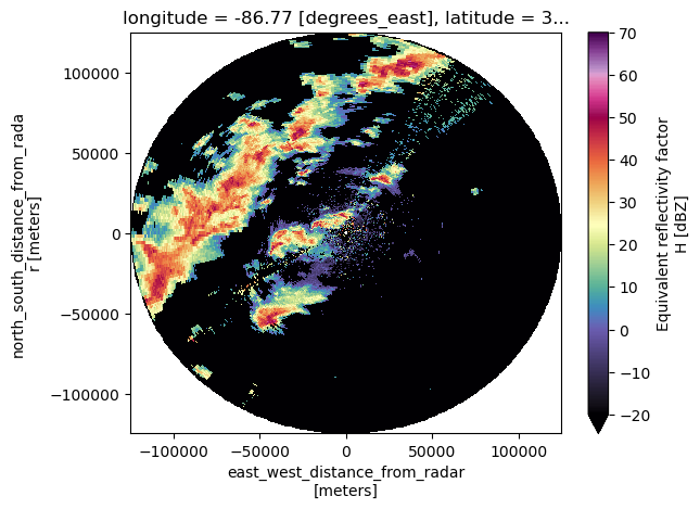
proj_crs = xd.georeference.get_crs(ds)
cart_crs = cartopy.crs.Projection(proj_crs)
fig = plt.figure(figsize=(10, 10))
ax = fig.add_subplot(111, projection=cartopy.crs.PlateCarree())
ds["DBZH"].plot(
x="x",
y="y",
cmap="ChaseSpectral",
transform=cart_crs,
cbar_kwargs=dict(pad=0.075, shrink=0.75),
vmin=-20,
vmax=70
)
ax.coastlines()
ax.gridlines(draw_labels=True)
/Users/mgrover/mambaforge/envs/ams-open-radar-2023-dev/lib/python3.10/site-packages/cartopy/mpl/geoaxes.py:1785: UserWarning: The input coordinates to pcolormesh are interpreted as cell centers, but are not monotonically increasing or decreasing. This may lead to incorrectly calculated cell edges, in which case, please supply explicit cell edges to pcolormesh.
result = super().pcolormesh(*args, **kwargs)
<cartopy.mpl.gridliner.Gridliner at 0x2d39cc2e0>
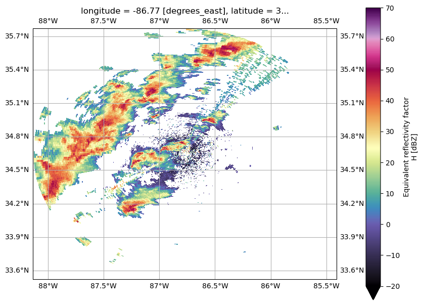
Slicing and Dicing Radar Data
Since we use the xarray.Dataset data structure here, we can make use of the subsetting interface!
Subset along Azimuth
Let’s start be selecting values along a given azimuth, or degrees around the radar. There are convective cells to the West (270 degrees), so we can start there. We need to specify method='nearest' in the case the value is not exactly what we are looking for.
subset_azimuth = ds.sel(azimuth=270,
method='nearest')
subset_azimuth
<xarray.Dataset>
Dimensions: (range: 992)
Coordinates:
azimuth float64 270.0
elevation float64 0.4614
time datetime64[ns] ...
* range (range) float32 1e+03 1.125e+03 ... 1.248e+05 1.249e+05
longitude float64 -86.77
latitude float64 34.65
altitude float64 200.0
spatial_ref int64 0
x (range) float64 -999.9 -1.125e+03 ... -1.248e+05
y (range) float64 0.04793 0.05393 0.05992 ... 5.979 5.985
z (range) float64 208.1 209.1 210.2 ... 2.12e+03 2.123e+03
Data variables: (12/13)
DBTH (range) float32 ...
DBZH (range) float64 nan nan nan nan nan ... nan nan nan nan
VRADH (range) float64 0.0 0.0 0.0 0.0 0.0 ... 0.0 0.0 0.0 0.0
WRADH (range) float32 ...
ZDR (range) float32 ...
KDP (range) float32 ...
... ...
RHOHV (range) float32 ...
sweep_mode <U20 ...
sweep_number int64 ...
prt_mode <U7 ...
follow_mode <U7 ...
sweep_fixed_angle float64 ...- range: 992
- azimuth()float64270.0
- standard_name :
- ray_azimuth_angle
- long_name :
- azimuth_angle_from_true_north
- units :
- degrees
- axis :
- radial_azimuth_coordinate
array(270.00274658)
- elevation()float640.4614
- standard_name :
- ray_elevation_angle
- long_name :
- elevation_angle_from_horizontal_plane
- units :
- degrees
- axis :
- radial_elevation_coordinate
array(0.461426)
- time()datetime64[ns]...
- standard_name :
- time
[1 values with dtype=datetime64[ns]]
- range(range)float321e+03 1.125e+03 ... 1.249e+05
- units :
- meters
- standard_name :
- projection_range_coordinate
- long_name :
- range_to_measurement_volume
- axis :
- radial_range_coordinate
- meters_between_gates :
- 6250.0
- spacing_is_constant :
- true
- meters_to_center_of_first_gate :
- 100000
array([ 1000., 1125., 1250., ..., 124625., 124750., 124875.], dtype=float32) - longitude()float64-86.77
- long_name :
- longitude
- units :
- degrees_east
- standard_name :
- longitude
array(-86.7715)
- latitude()float6434.65
- long_name :
- latitude
- units :
- degrees_north
- positive :
- up
- standard_name :
- latitude
array(34.6462)
- altitude()float64200.0
- long_name :
- altitude
- units :
- meters
- standard_name :
- altitude
array(200.)
- spatial_ref()int640
- crs_wkt :
- PROJCRS["unknown",BASEGEOGCRS["unknown",DATUM["World Geodetic System 1984",ELLIPSOID["WGS 84",6378137,298.257223563,LENGTHUNIT["metre",1]],ID["EPSG",6326]],PRIMEM["Greenwich",0,ANGLEUNIT["degree",0.0174532925199433],ID["EPSG",8901]]],CONVERSION["unknown",METHOD["Modified Azimuthal Equidistant",ID["EPSG",9832]],PARAMETER["Latitude of natural origin",34.6461999602616,ANGLEUNIT["degree",0.0174532925199433],ID["EPSG",8801]],PARAMETER["Longitude of natural origin",-86.7714999429882,ANGLEUNIT["degree",0.0174532925199433],ID["EPSG",8802]],PARAMETER["False easting",0,LENGTHUNIT["metre",1],ID["EPSG",8806]],PARAMETER["False northing",0,LENGTHUNIT["metre",1],ID["EPSG",8807]]],CS[Cartesian,2],AXIS["(E)",east,ORDER[1],LENGTHUNIT["metre",1,ID["EPSG",9001]]],AXIS["(N)",north,ORDER[2],LENGTHUNIT["metre",1,ID["EPSG",9001]]]]
- semi_major_axis :
- 6378137.0
- semi_minor_axis :
- 6356752.314245179
- inverse_flattening :
- 298.257223563
- reference_ellipsoid_name :
- WGS 84
- longitude_of_prime_meridian :
- 0.0
- prime_meridian_name :
- Greenwich
- geographic_crs_name :
- unknown
- horizontal_datum_name :
- World Geodetic System 1984
- projected_crs_name :
- unknown
- grid_mapping_name :
- azimuthal_equidistant
- latitude_of_projection_origin :
- 34.64619996026158
- longitude_of_projection_origin :
- -86.77149994298816
- false_easting :
- 0.0
- false_northing :
- 0.0
array(0)
- x(range)float64-999.9 -1.125e+03 ... -1.248e+05
- standard_name :
- east_west_distance_from_radar
- units :
- meters
array([ -999.94307597, -1124.93582579, -1249.92854549, -1374.92123503, -1499.91389436, -1624.90652341, -1749.89912213, -1874.89169047, -1999.88422838, -2124.87673581, -2249.86921268, -2374.86165897, -2499.8540746 , -2624.84645952, -2749.83881369, -2874.83113705, -2999.82342953, -3124.8156911 , -3249.80792169, -3374.80012125, -3499.79228972, -3624.78442706, -3749.77653321, -3874.76860811, -3999.76065171, -4124.75266396, -4249.7446448 , -4374.73659417, -4499.72851203, -4624.72039832, -4749.71225298, -4874.70407597, -4999.69586722, -5124.68762668, -5249.67935431, -5374.67105004, -5499.66271381, -5624.65434559, -5749.64594531, -5874.63751291, -5999.62904835, -6124.62055157, -6249.61202252, -6374.60346114, -6499.59486737, -6624.58624117, -6749.57758248, -6874.56889125, -6999.56016741, -7124.55141093, -7249.54262173, -7374.53379978, -7499.52494501, -7624.51605737, -7749.50713681, -7874.49818327, -7999.48919669, -8124.48017704, -8249.47112424, -8374.46203825, ... -117597.79018213, -117722.73132946, -117847.67239585, -117972.61338207, -118097.55428724, -118222.49511214, -118347.43585588, -118472.37651841, -118597.31710051, -118722.25760212, -118847.19802236, -118972.13836116, -119097.07861932, -119222.01879678, -119346.95889265, -119471.89890687, -119596.83884023, -119721.77869268, -119846.71846331, -119971.65815208, -120096.59775978, -120221.5372855 , -120346.47673004, -120471.4160925 , -120596.35537367, -120721.29457264, -120846.23369023, -120971.17272551, -121096.11167929, -121221.05055066, -121345.98934042, -121470.92804766, -121595.86667319, -121720.80521609, -121845.74367717, -121970.68205551, -122095.62035106, -122220.55856463, -122345.49669616, -122470.43474474, -122595.3727103 , -122720.31059367, -122845.24839479, -122970.18611274, -123095.12374747, -123220.06129978, -123344.99876963, -123469.93615609, -123594.8734591 , -123719.81067949, -123844.74781633, -123969.68487044, -124094.62184088, -124219.55872849, -124344.49553232, -124469.43225321, -124594.36889022, -124719.30544418, -124844.24191415]) - y(range)float640.04793 0.05393 ... 5.979 5.985
- standard_name :
- north_south_distance_from_radar
- units :
- meters
array([0.04793417, 0.05392594, 0.0599177 , 0.06590946, 0.07190122, 0.07789298, 0.08388474, 0.08987649, 0.09586825, 0.10186 , 0.10785175, 0.11384351, 0.11983525, 0.125827 , 0.13181875, 0.13781049, 0.14380223, 0.14979398, 0.15578572, 0.16177745, 0.16776919, 0.17376093, 0.17975266, 0.18574439, 0.19173613, 0.19772785, 0.20371958, 0.20971131, 0.21570303, 0.22169476, 0.22768648, 0.2336782 , 0.23966992, 0.24566164, 0.25165335, 0.25764507, 0.26363678, 0.26962849, 0.2756202 , 0.28161191, 0.28760362, 0.29359532, 0.29958702, 0.30557873, 0.31157043, 0.31756213, 0.32355382, 0.32954552, 0.33553721, 0.34152891, 0.3475206 , 0.35351229, 0.35950397, 0.36549566, 0.37148735, 0.37747903, 0.38347071, 0.38946239, 0.39545407, 0.40144575, 0.40743742, 0.4134291 , 0.41942077, 0.42541244, 0.43140411, 0.43739577, 0.44338744, 0.4493791 , 0.45537077, 0.46136243, 0.46735409, 0.47334574, 0.4793374 , 0.48532905, 0.49132071, 0.49731236, 0.50330401, 0.50929566, 0.5152873 , 0.52127895, 0.52727059, 0.53326223, 0.53925387, 0.54524551, 0.55123714, 0.55722878, 0.56322041, 0.56921204, 0.57520367, 0.5811953 , 0.58718693, 0.59317855, 0.59917017, 0.6051618 , 0.61115342, 0.61714503, 0.62313665, 0.62912826, 0.63511988, 0.64111149, ... 5.40967757, 5.415667 , 5.42165643, 5.42764586, 5.43363529, 5.43962471, 5.44561413, 5.45160354, 5.45759295, 5.46358235, 5.46957176, 5.47556115, 5.48155055, 5.48753994, 5.49352933, 5.49951871, 5.50550809, 5.51149746, 5.51748684, 5.5234762 , 5.52946557, 5.53545493, 5.54144429, 5.54743364, 5.55342299, 5.55941233, 5.56540167, 5.57139101, 5.57738034, 5.58336967, 5.589359 , 5.59534832, 5.60133764, 5.60732695, 5.61331626, 5.61930557, 5.62529487, 5.63128417, 5.63727347, 5.64326276, 5.64925205, 5.65524133, 5.66123061, 5.66721989, 5.67320916, 5.67919843, 5.68518769, 5.69117695, 5.69716621, 5.70315546, 5.70914471, 5.71513395, 5.72112319, 5.72711243, 5.73310166, 5.73909089, 5.74508012, 5.75106934, 5.75705856, 5.76304777, 5.76903698, 5.77502618, 5.78101539, 5.78700458, 5.79299378, 5.79898297, 5.80497215, 5.81096134, 5.81695051, 5.82293969, 5.82892886, 5.83491803, 5.84090719, 5.84689635, 5.8528855 , 5.85887465, 5.8648638 , 5.87085294, 5.87684208, 5.88283121, 5.88882035, 5.89480947, 5.9007986 , 5.90678771, 5.91277683, 5.91876594, 5.92475505, 5.93074415, 5.93673325, 5.94272234, 5.94871144, 5.95470052, 5.96068961, 5.96667868, 5.97266776, 5.97865683, 5.9846459 ]) - z(range)float64208.1 209.1 ... 2.12e+03 2.123e+03
- standard_name :
- height_above_ground
- units :
- meters
array([ 208.11216484, 209.13446161, 210.15859752, 211.18457257, 212.21238677, 213.24204011, 214.27353259, 215.30686421, 216.34203497, 217.37904487, 218.41789391, 219.45858209, 220.50110941, 221.54547587, 222.59168146, 223.63972619, 224.68961005, 225.74133305, 226.79489517, 227.85029644, 228.90753683, 229.96661636, 231.02753502, 232.09029281, 233.15488973, 234.22132571, 235.28960095, 236.35971519, 237.43166868, 238.50546117, 239.58109291, 240.65856366, 241.73787365, 242.81902264, 243.90201088, 244.98683812, 246.0735046 , 247.16201008, 248.25235479, 249.34453851, 250.43856147, 251.53442342, 252.63212461, 253.7316648 , 254.83304422, 255.93626264, 257.04132029, 258.14821694, 259.25695281, 260.36752769, 261.47994179, 262.59419488, 263.7102872 , 264.82821851, 265.94798905, 267.06959857, 268.19304733, 269.31833507, 270.44546179, 271.57442798, 272.70523315, 273.83787731, 274.97236045, 276.10868305, 277.24684463, 278.38684519, 279.52868474, 280.67236373, 281.81788171, 282.96523867, 284.1144346 , 285.26546999, 286.41834435, 287.57305769, 288.72961 , 289.88800176, 291.04823249, 292.2103022 , 293.37421088, 294.539959 , ... 1904.33886097, 1907.03800485, 1909.73901585, 1912.44189395, 1915.1465789 , 1917.8530707 , 1920.56142961, 1923.27165562, 1925.98368847, 1928.69758842, 1931.41329521, 1934.13080885, 1936.85018957, 1939.57143739, 1942.29449204, 1945.01941378, 1947.74614235, 1950.474738 , 1953.20514048, 1955.93741004, 1958.67148643, 1961.40742989, 1964.14518017, 1966.88479753, 1969.6262217 , 1972.36951294, 1975.114611 , 1977.86157612, 1980.61040831, 1983.3610473 , 1986.1134931 , 1988.86780596, 1991.62398588, 1994.3819726 , 1997.14176611, 1999.90342668, 2002.6669543 , 2005.43228871, 2008.19942991, 2010.96843816, 2013.73931346, 2016.51199553, 2019.28654465, 2022.06290055, 2024.84112349, 2027.6211532 , 2030.40304995, 2033.18675347, 2035.97232402, 2038.75970135, 2041.5489457 , 2044.33999681, 2047.13291495, 2049.92763985, 2052.72423177, 2055.52263045, 2058.32289615, 2061.12502886, 2063.92896832, 2066.73471453, 2069.54232776, 2072.35180799, 2075.16309497, 2077.97618869, 2080.79114941, 2083.60797713, 2086.42661159, 2089.2470528 , 2092.06936099, 2094.89353617, 2097.71951809, 2100.54736699, 2103.37702263, 2106.20854525, 2109.04187459, 2111.87707091, 2114.71407396, 2117.55294398, 2120.39362072, 2123.23616443])
- DBTH(range)float32...
- units :
- dBZ
- long_name :
- Total power H (uncorrected reflectivity)
- standard_name :
- radar_equivalent_reflectivity_factor_h
- coordinates :
- elevation azimuth range latitude longitude altitude time rtime sweep_mode
[992 values with dtype=float32]
- DBZH(range)float64nan nan nan nan ... nan nan nan nan
- units :
- dBZ
- long_name :
- Equivalent reflectivity factor H
- standard_name :
- radar_equivalent_reflectivity_factor_h
- coordinates :
- elevation azimuth range latitude longitude altitude time rtime sweep_mode
array([ nan, nan, nan, nan, nan, nan, nan, nan, nan, nan, nan, nan, nan, nan, nan, nan, nan, nan, nan, nan, nan, nan, nan, nan, 30. , 40.5, nan, nan, nan, nan, 4. , 16. , 4. , -4. , -11.5, 2.5, 9. , -7. , -12. , -14.5, -12. , -15.5, -17. , -15. , -11. , nan, nan, nan, nan, nan, nan, nan, -14. , -7.5, 8.5, -6.5, -3. , nan, nan, nan, nan, 13.5, 12.5, nan, nan, nan, 2.5, -6. , -5. , -5. , -2.5, -1.5, 8. , 1.5, 0. , nan, -2. , -1. , -6.5, -2.5, 4. , -2. , 6. , 7.5, 1.5, 3.5, 4. , 3.5, 1. , -1. , 5. , 2.5, 4. , 3. , 4.5, 4. , 4.5, 4.5, 9.5, 8.5, 4. , 7. , 4.5, 3.5, 4. , 0.5, 1.5, 3. , 3.5, 2.5, 3.5, 7.5, 8. , 6.5, 10. , 8.5, 10. , 11.5, 10.5, 8. , 12.5, 9.5, 10.5, 10. , 9. , 10. , 10. , 13. , 9. , 8.5, 7.5, 12.5, 11.5, 12. , 13.5, 11. , 10.5, 13.5, 10. , 12.5, 13. , 10. , 12. , 10. , 8.5, 8.5, 8. , 4. , 1.5, -3. , 0. , 0. , -0.5, 2. , 2. , 0.5, -1. , -1.5, -1. , 0.5, -1. , 3. , 4.5, 6. , 5. , 8.5, 5. , 6. , 8. , 9. , 10. , 7.5, 7.5, 8. , 9.5, 9. , 8.5, 8.5, 8. , 8.5, ... 15. , 13.5, 15. , 16.5, 17. , 14. , 14. , 14.5, 11.5, 11.5, 11. , 11.5, 11. , 9. , 8. , 5. , 7.5, 7. , 8. , 6. , 5.5, 9. , 7. , 7. , 9.5, 10. , 6. , 10. , 7.5, 9.5, 12. , 8.5, 9.5, 15. , 15. , 13.5, 8. , 7.5, 4. , 3.5, 6.5, 4.5, 8. , 6. , 5.5, 8.5, 7.5, 6. , 8.5, 11. , 16. , 12. , 8.5, 10. , 9. , 8. , 8. , 5.5, 13. , 12.5, 10. , 5. , 4. , 7. , 6. , 5.5, 7.5, 7.5, 4. , 7. , 6. , 7. , 7.5, 7.5, 6. , 5.5, 5.5, 6. , 6. , 4.5, 5. , 4.5, 14.5, 15.5, 14.5, 12.5, 4.5, 4.5, 4.5, 11.5, 7.5, 4. , 4.5, 5. , 6. , 7.5, 5.5, 7.5, 8. , 13.5, 14.5, 13.5, 15.5, 14.5, 15. , 13. , 18. , 17. , 21.5, 22.5, 21. , 15. , 14. , 13. , 12. , 9.5, 8. , 4.5, 6. , nan, nan, nan, nan, nan, nan, nan, nan, nan, nan, nan, nan, nan, nan, nan, nan, nan, nan, nan, nan, nan, nan, nan, nan, nan, nan, 5.5, 6. , 5. , 5. , 13. , 8. , 6.5, 9.5, 9. , 7.5, 8.5, 8. , 9. , 9.5, 13. , 8.5, 8.5, 7. , 10.5, 10. , 9. , 6. , 7.5, 5.5, nan, nan, nan, nan]) - VRADH(range)float640.0 0.0 0.0 0.0 ... 0.0 0.0 0.0 0.0
- units :
- meters per seconds
- long_name :
- Radial velocity of scatterers away from instrument H
- standard_name :
- radial_velocity_of_scatterers_away_from_instrument_h
- coordinates :
- elevation azimuth range latitude longitude altitude time rtime sweep_mode
masked_array(data=[--, --, --, ..., --, --, --], mask=[ True, True, True, ..., True, True, True], fill_value=0) - WRADH(range)float32...
- units :
- meters per seconds
- long_name :
- Doppler spectrum width H
- standard_name :
- radar_doppler_spectrum_width_h
- coordinates :
- elevation azimuth range latitude longitude altitude time rtime sweep_mode
[992 values with dtype=float32]
- ZDR(range)float32...
- units :
- dB
- long_name :
- Log differential reflectivity H/V
- standard_name :
- radar_differential_reflectivity_hv
- coordinates :
- elevation azimuth range latitude longitude altitude time rtime sweep_mode
[992 values with dtype=float32]
- KDP(range)float32...
- units :
- degrees per kilometer
- long_name :
- Specific differential phase HV
- standard_name :
- radar_specific_differential_phase_hv
- coordinates :
- elevation azimuth range latitude longitude altitude time rtime sweep_mode
[992 values with dtype=float32]
- PHIDP(range)float32...
- units :
- degrees
- long_name :
- Differential phase HV
- standard_name :
- radar_differential_phase_hv
- coordinates :
- elevation azimuth range latitude longitude altitude time rtime sweep_mode
[992 values with dtype=float32]
- RHOHV(range)float32...
- units :
- unitless
- long_name :
- Correlation coefficient HV
- standard_name :
- radar_correlation_coefficient_hv
- coordinates :
- elevation azimuth range latitude longitude altitude time rtime sweep_mode
[992 values with dtype=float32]
- sweep_mode()<U20...
[1 values with dtype=<U20]
- sweep_number()int64...
[1 values with dtype=int64]
- prt_mode()<U7...
[1 values with dtype=<U7]
- follow_mode()<U7...
[1 values with dtype=<U7]
- sweep_fixed_angle()float64...
[1 values with dtype=float64]
- rangePandasIndex
PandasIndex(Float64Index([ 1000.0, 1125.0, 1250.0, 1375.0, 1500.0, 1625.0, 1750.0, 1875.0, 2000.0, 2125.0, ... 123750.0, 123875.0, 124000.0, 124125.0, 124250.0, 124375.0, 124500.0, 124625.0, 124750.0, 124875.0], dtype='float64', name='range', length=992))
subset_azimuth.DBZH.plot()
[<matplotlib.lines.Line2D at 0x2dafea800>]
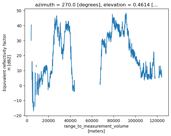
Subset Along the Range Dimension
We can follow a similar process for the range. Let’s select from near the radar (0 meters from the radar) to 50 km (50_000 meters) from the radar.
subset_range = ds.sel(range=slice(0, 50_000))
subset_range
<xarray.Dataset>
Dimensions: (azimuth: 360, range: 393)
Coordinates:
* azimuth (azimuth) float64 0.03296 1.033 1.994 ... 358.0 359.1
elevation (azimuth) float64 0.4614 0.4614 0.4614 ... 0.4614 0.4614
time (azimuth) datetime64[ns] ...
* range (range) float32 1e+03 1.125e+03 ... 4.988e+04 5e+04
longitude float64 -86.77
latitude float64 34.65
altitude float64 200.0
spatial_ref int64 0
x (azimuth, range) float64 0.5752 0.6471 ... -803.2 -805.2
y (azimuth, range) float64 999.9 1.125e+03 ... 4.999e+04
z (azimuth, range) float64 208.1 209.1 ... 748.0 749.8
Data variables: (12/13)
DBTH (azimuth, range) float32 ...
DBZH (azimuth, range) float64 nan nan nan nan ... nan nan nan
VRADH (azimuth, range) float64 0.0 0.0 0.0 0.0 ... 0.0 0.0 0.0
WRADH (azimuth, range) float32 ...
ZDR (azimuth, range) float32 ...
KDP (azimuth, range) float32 ...
... ...
RHOHV (azimuth, range) float32 ...
sweep_mode <U20 ...
sweep_number int64 ...
prt_mode <U7 ...
follow_mode <U7 ...
sweep_fixed_angle float64 ...- azimuth: 360
- range: 393
- azimuth(azimuth)float640.03296 1.033 1.994 ... 358.0 359.1
- standard_name :
- ray_azimuth_angle
- long_name :
- azimuth_angle_from_true_north
- units :
- degrees
- axis :
- radial_azimuth_coordinate
array([3.295898e-02, 1.032715e+00, 1.994019e+00, ..., 3.569980e+02, 3.580142e+02, 3.590771e+02]) - elevation(azimuth)float640.4614 0.4614 ... 0.4614 0.4614
- standard_name :
- ray_elevation_angle
- long_name :
- elevation_angle_from_horizontal_plane
- units :
- degrees
- axis :
- radial_elevation_coordinate
array([0.461426, 0.461426, 0.461426, ..., 0.461426, 0.461426, 0.461426])
- time(azimuth)datetime64[ns]...
- standard_name :
- time
[360 values with dtype=datetime64[ns]]
- range(range)float321e+03 1.125e+03 ... 4.988e+04 5e+04
- units :
- meters
- standard_name :
- projection_range_coordinate
- long_name :
- range_to_measurement_volume
- axis :
- radial_range_coordinate
- meters_between_gates :
- 6250.0
- spacing_is_constant :
- true
- meters_to_center_of_first_gate :
- 100000
array([ 1000., 1125., 1250., ..., 49750., 49875., 50000.], dtype=float32)
- longitude()float64-86.77
- long_name :
- longitude
- units :
- degrees_east
- standard_name :
- longitude
array(-86.7715)
- latitude()float6434.65
- long_name :
- latitude
- units :
- degrees_north
- positive :
- up
- standard_name :
- latitude
array(34.6462)
- altitude()float64200.0
- long_name :
- altitude
- units :
- meters
- standard_name :
- altitude
array(200.)
- spatial_ref()int640
- crs_wkt :
- PROJCRS["unknown",BASEGEOGCRS["unknown",DATUM["World Geodetic System 1984",ELLIPSOID["WGS 84",6378137,298.257223563,LENGTHUNIT["metre",1]],ID["EPSG",6326]],PRIMEM["Greenwich",0,ANGLEUNIT["degree",0.0174532925199433],ID["EPSG",8901]]],CONVERSION["unknown",METHOD["Modified Azimuthal Equidistant",ID["EPSG",9832]],PARAMETER["Latitude of natural origin",34.6461999602616,ANGLEUNIT["degree",0.0174532925199433],ID["EPSG",8801]],PARAMETER["Longitude of natural origin",-86.7714999429882,ANGLEUNIT["degree",0.0174532925199433],ID["EPSG",8802]],PARAMETER["False easting",0,LENGTHUNIT["metre",1],ID["EPSG",8806]],PARAMETER["False northing",0,LENGTHUNIT["metre",1],ID["EPSG",8807]]],CS[Cartesian,2],AXIS["(E)",east,ORDER[1],LENGTHUNIT["metre",1,ID["EPSG",9001]]],AXIS["(N)",north,ORDER[2],LENGTHUNIT["metre",1,ID["EPSG",9001]]]]
- semi_major_axis :
- 6378137.0
- semi_minor_axis :
- 6356752.314245179
- inverse_flattening :
- 298.257223563
- reference_ellipsoid_name :
- WGS 84
- longitude_of_prime_meridian :
- 0.0
- prime_meridian_name :
- Greenwich
- geographic_crs_name :
- unknown
- horizontal_datum_name :
- World Geodetic System 1984
- projected_crs_name :
- unknown
- grid_mapping_name :
- azimuthal_equidistant
- latitude_of_projection_origin :
- 34.64619996026158
- longitude_of_projection_origin :
- -86.77149994298816
- false_easting :
- 0.0
- false_northing :
- 0.0
array(0)
- x(azimuth, range)float640.5752 0.6471 ... -803.2 -805.2
- standard_name :
- east_west_distance_from_radar
- units :
- meters
array([[ 5.75210019e-01, 6.47111194e-01, 7.19012352e-01, ..., 2.86150491e+01, 2.86869411e+01, 2.87588332e+01], [ 1.80222724e+01, 2.02750540e+01, 2.25278351e+01, ..., 8.96556374e+02, 8.98808870e+02, 9.01061366e+02], [ 3.47931836e+01, 3.91423268e+01, 4.34914690e+01, ..., 1.73086112e+03, 1.73520971e+03, 1.73955830e+03], ..., [-5.23680806e+01, -5.89140837e+01, -6.54600851e+01, ..., -2.60516185e+03, -2.61170702e+03, -2.61825219e+03], [-3.46494678e+01, -3.89806466e+01, -4.33118243e+01, ..., -1.72371167e+03, -1.72804230e+03, -1.73237292e+03], [-1.61051850e+01, -1.81183310e+01, -2.01314765e+01, ..., -8.01186776e+02, -8.03199667e+02, -8.05212556e+02]]) - y(azimuth, range)float64999.9 1.125e+03 ... 4.999e+04
- standard_name :
- north_south_distance_from_radar
- units :
- meters
array([[ 999.94291168, 1124.93564096, 1249.92834012, ..., 49744.29260124, 49869.2694842 , 49994.24631596], [ 999.78065353, 1124.75310057, 1249.72551749, ..., 49736.2207238 , 49861.17732708, 49986.13387917], [ 999.33757653, 1124.25463899, 1249.17167137, ..., 49714.17891325, 49839.08013899, 49963.98131356], ..., [ 998.57084957, 1123.39207127, 1248.2132629 , ..., 49676.03644564, 49800.84184276, 49925.64718876], [ 999.34256983, 1124.26025645, 1249.17791299, ..., 49714.42731552, 49839.32916534, 49964.23096399], [ 999.81337283, 1124.78990977, 1249.76641661, ..., 49737.84841516, 49862.80910783, 49987.76974931]]) - z(azimuth, range)float64208.1 209.1 210.2 ... 748.0 749.8
- standard_name :
- height_above_ground
- units :
- meters
array([[208.11216484, 209.13446161, 210.15859752, ..., 746.30855122, 748.04805187, 749.78939026], [208.11216484, 209.13446161, 210.15859752, ..., 746.30855122, 748.04805187, 749.78939026], [208.11216484, 209.13446161, 210.15859752, ..., 746.30855122, 748.04805187, 749.78939026], ..., [208.11216484, 209.13446161, 210.15859752, ..., 746.30855122, 748.04805187, 749.78939026], [208.11216484, 209.13446161, 210.15859752, ..., 746.30855122, 748.04805187, 749.78939026], [208.11216484, 209.13446161, 210.15859752, ..., 746.30855122, 748.04805187, 749.78939026]])
- DBTH(azimuth, range)float32...
- units :
- dBZ
- long_name :
- Total power H (uncorrected reflectivity)
- standard_name :
- radar_equivalent_reflectivity_factor_h
- coordinates :
- elevation azimuth range latitude longitude altitude time rtime sweep_mode
[141480 values with dtype=float32]
- DBZH(azimuth, range)float64nan nan nan nan ... nan nan nan nan
- units :
- dBZ
- long_name :
- Equivalent reflectivity factor H
- standard_name :
- radar_equivalent_reflectivity_factor_h
- coordinates :
- elevation azimuth range latitude longitude altitude time rtime sweep_mode
array([[nan, nan, nan, ..., nan, nan, nan], [nan, nan, nan, ..., nan, nan, nan], [nan, nan, nan, ..., nan, nan, nan], ..., [nan, nan, 19., ..., nan, nan, nan], [nan, nan, 20., ..., nan, nan, nan], [nan, nan, nan, ..., nan, nan, nan]]) - VRADH(azimuth, range)float640.0 0.0 0.0 0.0 ... 0.0 0.0 0.0 0.0
- units :
- meters per seconds
- long_name :
- Radial velocity of scatterers away from instrument H
- standard_name :
- radial_velocity_of_scatterers_away_from_instrument_h
- coordinates :
- elevation azimuth range latitude longitude altitude time rtime sweep_mode
masked_array( data=[[--, --, --, ..., --, --, --], [--, --, --, ..., --, --, --], [--, --, --, ..., --, --, --], ..., [--, --, -2.532283464566929, ..., --, --, --], [--, --, -1.7725984251968503, ..., --, --, --], [--, --, --, ..., --, --, --]], mask=[[ True, True, True, ..., True, True, True], [ True, True, True, ..., True, True, True], [ True, True, True, ..., True, True, True], ..., [ True, True, False, ..., True, True, True], [ True, True, False, ..., True, True, True], [ True, True, True, ..., True, True, True]], fill_value=0) - WRADH(azimuth, range)float32...
- units :
- meters per seconds
- long_name :
- Doppler spectrum width H
- standard_name :
- radar_doppler_spectrum_width_h
- coordinates :
- elevation azimuth range latitude longitude altitude time rtime sweep_mode
[141480 values with dtype=float32]
- ZDR(azimuth, range)float32...
- units :
- dB
- long_name :
- Log differential reflectivity H/V
- standard_name :
- radar_differential_reflectivity_hv
- coordinates :
- elevation azimuth range latitude longitude altitude time rtime sweep_mode
[141480 values with dtype=float32]
- KDP(azimuth, range)float32...
- units :
- degrees per kilometer
- long_name :
- Specific differential phase HV
- standard_name :
- radar_specific_differential_phase_hv
- coordinates :
- elevation azimuth range latitude longitude altitude time rtime sweep_mode
[141480 values with dtype=float32]
- PHIDP(azimuth, range)float32...
- units :
- degrees
- long_name :
- Differential phase HV
- standard_name :
- radar_differential_phase_hv
- coordinates :
- elevation azimuth range latitude longitude altitude time rtime sweep_mode
[141480 values with dtype=float32]
- RHOHV(azimuth, range)float32...
- units :
- unitless
- long_name :
- Correlation coefficient HV
- standard_name :
- radar_correlation_coefficient_hv
- coordinates :
- elevation azimuth range latitude longitude altitude time rtime sweep_mode
[141480 values with dtype=float32]
- sweep_mode()<U20...
[1 values with dtype=<U20]
- sweep_number()int64...
[1 values with dtype=int64]
- prt_mode()<U7...
[1 values with dtype=<U7]
- follow_mode()<U7...
[1 values with dtype=<U7]
- sweep_fixed_angle()float64...
[1 values with dtype=float64]
- azimuthPandasIndex
PandasIndex(Float64Index([ 0.032958984375, 1.03271484375, 1.9940185546875, 3.06793212890625, 4.04571533203125, 5.0482177734375, 6.0260009765625, 7.064208984375, 8.0364990234375, 9.0472412109375, ... 350.05462646484375, 351.02142333984375, 352.0513916015625, 353.0621337890625, 354.0509033203125, 355.00396728515625, 356.09161376953125, 356.99798583984375, 358.01422119140625, 359.0771484375], dtype='float64', name='azimuth', length=360)) - rangePandasIndex
PandasIndex(Float64Index([ 1000.0, 1125.0, 1250.0, 1375.0, 1500.0, 1625.0, 1750.0, 1875.0, 2000.0, 2125.0, ... 48875.0, 49000.0, 49125.0, 49250.0, 49375.0, 49500.0, 49625.0, 49750.0, 49875.0, 50000.0], dtype='float64', name='range', length=393))
Plot a PPI of the Range Subset
fig = plt.figure(figsize=(10, 10))
ax = fig.add_subplot(111, projection=cartopy.crs.PlateCarree())
subset_range["DBZH"].plot(
x="x",
y="y",
cmap="ChaseSpectral",
transform=cart_crs,
cbar_kwargs=dict(pad=0.075, shrink=0.75),
vmin=-20,
vmax=70
)
ax.coastlines()
ax.gridlines(draw_labels=True)
/Users/mgrover/mambaforge/envs/ams-open-radar-2023-dev/lib/python3.10/site-packages/cartopy/mpl/geoaxes.py:1785: UserWarning: The input coordinates to pcolormesh are interpreted as cell centers, but are not monotonically increasing or decreasing. This may lead to incorrectly calculated cell edges, in which case, please supply explicit cell edges to pcolormesh.
  result = super().pcolormesh(*args, **kwargs)
<cartopy.mpl.gridliner.Gridliner at 0x2db2d5de0>
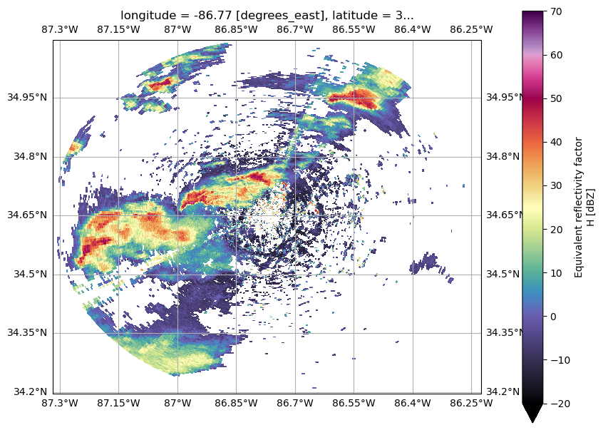
# some subsection code
new = "helpful information"
Summary
Within this notebook, we took a look at the basics of the xradar package, and how it enables us to use the xarray ecosystem. The process from reading the data, applying filtering, subsetting, and visualizing the data was covered. We encourage users to explore the rest of the xradar user guide to continue learning how this tool is useful for their workflows.