Interaction of BALTRAD and wradlib via ODIM_H5
Prepare your environment
%matplotlib inline
import numpy as np
import matplotlib.pyplot as plt
from matplotlib.patches import Polygon
from matplotlib.collections import PatchCollection
import matplotlib.ticker as mticker
import wradlib
import shapefile
import gc
/srv/conda/envs/notebook/lib/python3.9/site-packages/requests/__init__.py:102: RequestsDependencyWarning: urllib3 (1.26.8) or chardet (5.2.0)/charset_normalizer (2.0.10) doesn't match a supported version!
  warnings.warn("urllib3 ({}) or chardet ({})/charset_normalizer ({}) doesn't match a supported "
Run BALTRAD’s odc_toolbox
First, you will process a scan from Suergavere (Estland) by using BALTRAD’s odc_toolbox.
From your VM’s vagrant directory, navigate to the folder /baltrad2wradlib.
Execute the following command:
$ odc_toolbox -i in -o out -q ropo,radvol-att
Check whether a file was created in the folder /out.
BALTRAD will not create output files if these already exist. You can check that via !ls out.
!odc_toolbox -i in -o out -q ropo,radvol-att
Exception ignored in: <function _after_at_fork_child_reinit_locks at 0x7fa6e2f18820>
Traceback (most recent call last):
  File "/srv/conda/envs/notebook/lib/python3.9/logging/__init__.py", line 255, in _after_at_fork_child_reinit_locks
    handler._at_fork_reinit()
  File "/srv/conda/envs/notebook/lib/python3.9/logging/__init__.py", line 894, in _at_fork_reinit
    self.lock._at_fork_reinit()
AttributeError: 'RLock' object has no attribute '_at_fork_reinit'
Objects created: 1509
Objects deleted: 1509
Objects pending: 0
!ls out
201405190715_SUR.h5
Read and inspect data from Suergavere (Estonia) before and after QC with odc_toolbox
# Before QC
inp = wradlib.io.read_opera_hdf5("in/201405190715_SUR.h5")
# After QC
out = wradlib.io.read_opera_hdf5("out/201405190715_SUR.h5")
# Here you can inspect whichever directory you want, e.g.
print("where...\n", inp['where'],"\n")
print("what...\n", inp['what'],"\n")
print("dataset1/data1/what...\n", inp['dataset1/data1/what'])
where...
 {'height': 157.0, 'lat': 58.482310026884086, 'lon': 25.518660116940737, 'towerheight': 29.0}

what...
 {'date': b'20140519', 'object': b'PVOL', 'source': b'WMO:26232,RAD:EE41,PLC:S\xc3\xbcrgavere,NOD:eesur', 'time': b'071500', 'version': b'H5rad 2.2'}

dataset1/data1/what...
 {'gain': 0.5, 'nodata': 255.0, 'offset': -32.0, 'quantity': b'DBZH', 'undetect': 0.0}
Convert selected fields to target units
def convert(dset, dir):
    """Converts ODIM_H5 data representations to values in target unit and masks missing values.

    Parameters
    ----------
    dset : the hdf5 object returned by wradlib.read_OPERA_hdf5
    dir : the corresponding directory tree in dset for which the data should be processed

    """
    res = dset[dir+"/data"].astype(np.uint16)
    try:
        res = res * dset[dir+"/what"]["gain"] + dset[dir+"/what"]["offset"]
    except:
        pass
    try:
        res[dset[dir+"/data"]==dset[dir+"/what"]["nodata"]] = np.nan
    except:
        pass
    try:
        res[dset[dir+"/data"]==dset[dir+"/what"]["undetect"]] = np.nan
    except:
        pass

    return res
# Extract specific data arrays from ODIM_h5 objects
#    dBZH before QC
before= convert(inp, "dataset1/data1")
#    dBZH after QC
after = convert(out, "dataset1/data1")
#    Quality field 1
qual1 = convert(out, "dataset1/quality1")
#    Quality field 2
qual2 = convert(out, "dataset1/quality2")
Collect all the information required for georeferencing
# Collect all the georeferencing information we need
#   First gate
r0 = inp['dataset1/where']["rstart"]*1000.
#   Gate length
rscale = inp['dataset1/where']["rscale"]
#   Number of bins per beam
nbins = inp['dataset1/where']["nbins"]
#   Maximum range
maxr = r0 + (nbins)*rscale
# Construct array of range gates
r = np.linspace(r0, maxr, nbins)
# Construct array of azimuth angles (quick and dirty)
az = np.linspace(0, 359, inp['dataset1/where']["nrays"])
# Site coordinates (lon,lat)
site = (inp["where"]["lon"], inp["where"]["lat"], inp["where"]["height"])
# Define a projection (Azimuthal Equidistant)
proj = wradlib.georef.create_osr("aeqd", lon_0=site[0], lat_0=site[1])
Design a plot we will use for all PPIs in this exercise
# A little helper funciton to harmonize all plots
def plot_ppi_to_ax(ppi, ax, title="", cb=True, cb_label="", cb_shrink=0.75, bbox=[-maxr, maxr, -maxr, maxr], extend="min", **kwargs):
    """This is the function that we use in this exercise to plot PPIs with uniform georeferencing and style.
    """
    # Read, project and plot country shapefile as background
    # (got that snippet from http://stackoverflow.com/questions/15968762/shapefile-and-matplotlib-plot-polygon-collection-of-shapefile-coordinates)
    sf = shapefile.Reader("shp/europe_countries.shp", encoding="latin1")
    recs    = sf.records()
    shapes  = sf.shapes()
    Nshp    = len(shapes)
    # Iterate over shapes and create matplotlib Polygons
    for nshp in range(Nshp):
        ptchs   = []
        pts     = np.array(shapes[nshp].points)
        pts = wradlib.georef.reproject(pts, projection_target=proj)
        prt     = shapes[nshp].parts
        par     = list(prt) + [pts.shape[0]]
        for pij in range(len(prt)):
            ptchs.append(Polygon(pts[par[pij]:par[pij+1]]))
        ax.add_collection(PatchCollection(ptchs,facecolor="lightgrey",edgecolor='k', linewidths=1, zorder=-1))


    # use wradlib.vis.plot_ppi
    ax, pm = wradlib.vis.plot_ppi(np.ma.masked_invalid(ppi), ax=ax, r=r, az=az, site=site, proj=proj, **kwargs)
    # and plot a cross hair
    ax = wradlib.vis.plot_ppi_crosshair(site=site, ranges=[50000, 100000,150000, 200000, maxr], angles=[0, 90, 180, 270],
                                        proj=proj, elev=0.5, ax=ax)
    ##plt.text(x=-244000, y=-60000,s="250km", color="gray", rotation=-69)
    ##plt.text(x=-192000, y=-60000,s="200km", color="gray", rotation=-67)
    ##plt.text(x=-138000, y=-60000,s="150km", color="gray", rotation=-65)


    # Do our final decorations
    plt.xlim(bbox[0], bbox[1])
    plt.ylim(bbox[2], bbox[3])
    # set title
    plt.title(title)
    # convert axes unit from meters to kilometers
    xticks_loc = ax.get_xticks().tolist()
    yticks_loc = ax.get_yticks().tolist()
    ax.xaxis.set_major_locator(mticker.FixedLocator(xticks_loc))
    ax.yaxis.set_major_locator(mticker.FixedLocator(yticks_loc))
    ax.set_xticklabels(['%g' % (0.001*l) for l in ax.get_xticks()])
    ax.set_yticklabels(['%g' % (0.001*l) for l in ax.get_yticks()])
    # set axes lables
    plt.xlabel("x coordinates (km)", fontsize="large")
    plt.ylabel("y coordinates (km)", fontsize="large")
    # plot colorbar
    if cb:
        cbar = plt.colorbar(pm, shrink=cb_shrink, orientation="horizontal", extend=extend, pad=0.1)
        cbar.set_label(cb_label, fontsize="large")

    gc.collect()

    return ax, pm
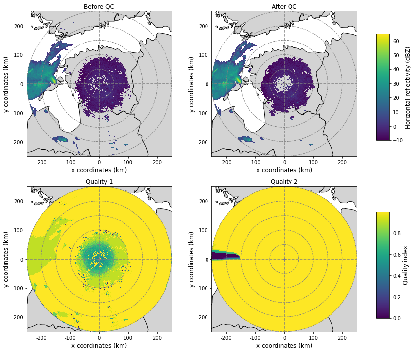
Plot the selected fields into one figure
fig = plt.figure(figsize=(12,10))

ax = plt.subplot(221, aspect="equal")
ax, pm = plot_ppi_to_ax(before, ax=ax, title="Before QC", cb=False, vmin=-10, vmax=65)

ax = plt.subplot(222, aspect="equal")
ax, pm = plot_ppi_to_ax(after,  ax=ax, title="After QC",  cb=False, vmin=-10, vmax=65)

ax = plt.subplot(223, aspect="equal")
ax, qm = plot_ppi_to_ax(qual1,  ax=ax, title="Quality 1", cb=False)

ax = plt.subplot(224, aspect="equal")
ax, qm = plot_ppi_to_ax(qual2,  ax=ax, title="Quality 2", cb=False)

plt.tight_layout()

# Add colorbars
fig.subplots_adjust(right=0.9)
cax = fig.add_axes((0.9, 0.6, 0.03, 0.3))
cbar = plt.colorbar(pm, cax=cax)
cbar.set_label("Horizontal reflectivity (dBZ)", fontsize="large")

cax = fig.add_axes((0.9, 0.1, 0.03, 0.3))
cbar = plt.colorbar(qm, cax=cax)
cbar.set_label("Quality index", fontsize="large")
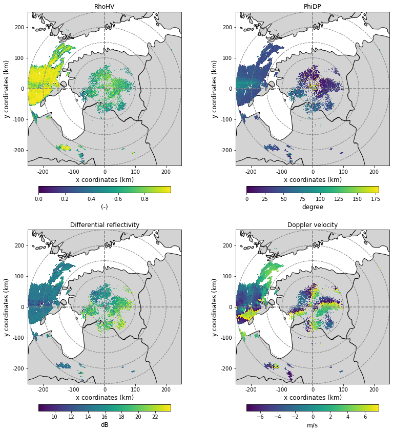
Collect and plot the polarimetric moments from the original ODIM_H5 dataset
# We organise the moments as a dictionary
moments = {}
moments["rho"] = convert(inp, "dataset1/data2")     # RhoHV
moments["phi"] = convert(inp, "dataset1/data4")     # PhiDP
moments["zdr"] = convert(inp, "dataset1/data5")     # ZDR - the value range is not plausible, is it? What went wrong?
moments["dop"] = convert(inp, "dataset1/data10")    # Doppler velocity
fig = plt.figure(figsize=(12,12))

ax = plt.subplot(221, aspect="equal")
ax, pm = plot_ppi_to_ax(moments["rho"], ax=ax, title="RhoHV", cb_label="(-)", cb_shrink=0.6, extend="neither")

ax = plt.subplot(222, aspect="equal")
ax, pm = plot_ppi_to_ax(moments["phi"], ax=ax, title="PhiDP", cb_label="degree", cb_shrink=0.6, extend="neither")

ax = plt.subplot(223, aspect="equal")
ax, pm = plot_ppi_to_ax(moments["zdr"], ax=ax, title="Differential reflectivity", cb_label="dB", cb_shrink=0.6, extend="neither")

ax = plt.subplot(224, aspect="equal")
ax, pm = plot_ppi_to_ax(moments["dop"], ax=ax, title="Doppler velocity", cb_label="m/s", cb_shrink=0.6, extend="neither")

plt.tight_layout()
Try some filtering and attenuation correction
# Set ZH to a very low value where we do not expect valid data
zh_filtered = np.where(np.isnan(before), -32., before)
# Retrieve PIA by using some constraints (see http://wradlib.bitbucket.org/atten.html for help)
pia = wradlib.atten.correct_attenuation_constrained(zh_filtered,
                                                  constraints=[wradlib.atten.constraint_dbz,
                                                               wradlib.atten.constraint_pia],
                                                  constraint_args=[[64.0],
                                                                   [20.0]])
# Correct reflectivity by PIA
after2 = before + pia
# Mask out non-meteorological echoes
after2[np.isnan(before)] = np.nan
/srv/conda/envs/notebook/lib/python3.9/site-packages/wradlib/trafo.py:261: RuntimeWarning: overflow encountered in power
  return 10.0 ** (x / 10.0)
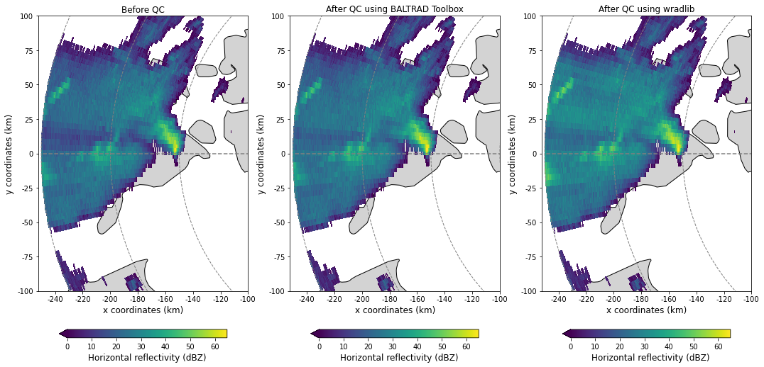
Compare results against QC from odc_toolbox
fig = plt.figure(figsize=(18,10))
bbox = [-maxr-2000,-100000, -100000, 100000]
shrink = 0.8

ax = plt.subplot(131, aspect="equal")
ax, pm = plot_ppi_to_ax(before, ax=ax, title="Before QC", cb_label="Horizontal reflectivity (dBZ)",
                        cb_shrink=shrink, bbox=bbox, vmin=0, vmax=65)


ax = plt.subplot(132, aspect="equal")
ax, pm = plot_ppi_to_ax(after,  ax=ax, title="After QC using BALTRAD Toolbox", cb_label="Horizontal reflectivity (dBZ)",
                        cb_shrink=shrink, bbox=bbox, vmin=0, vmax=65)


ax = plt.subplot(133, aspect="equal")
ax, pm = plot_ppi_to_ax(after2, ax=ax, title="After QC using wradlib", cb_label="Horizontal reflectivity (dBZ)",
                        cb_shrink=shrink, bbox=bbox, vmin=0, vmax=65)