![]()
wradlib Phase Processing - System PhiDP - ZPHI-Method
Overview
Within this notebook, we will cover:
Reading sweep data into xarray based Dataset
Retrieval of system PhiDP
ZPHI Phase processing
Attenuation correction using specific Attenuation
Prerequisites
Concepts |
Importance |
Notes |
|---|---|---|
Helpful |
Basic Dataset/DataArray |
|
Helpful |
Basic Plotting |
|
Helpful |
Projections |
Time to learn: 10 minutes
import datetime as dt
import glob
import os
import sys
import warnings

import matplotlib as mpl
import matplotlib.pyplot as plt
import numpy as np
import xarray as xr
from scipy.integrate import cumulative_trapezoid

import wradlib as wrl
/srv/conda/envs/notebook/lib/python3.9/site-packages/requests/__init__.py:102: RequestsDependencyWarning: urllib3 (1.26.8) or chardet (5.2.0)/charset_normalizer (2.0.10) doesn't match a supported version!
  warnings.warn("urllib3 ({}) or chardet ({})/charset_normalizer ({}) doesn't match a supported "
Import data
As a quick example to show the algorithm, we use a file from Down Under. For the further processing we us XBand data from BoXPol research radar at the University of Bonn, Germany.
boxpol = "data/hdf5/boxpol/2014-11-16--03:45:00,00.mvol"
terrey = "data/hdf5/terrey_39.h5"
swp0 = wrl.io.open_odim_dataset(terrey)[0]
swp0 = swp0.pipe(wrl.georef.georeference_dataset)
Pre-Processing
System PHIDP aka Phase Offset
The following function returns phase offset as well as start and stop ranges of the region of interest (first precipitating bins).
def phase_offset(phioff, method=None, rng=3000.0, npix=None, **kwargs):
    """Calculate Phase offset.

    Parameter
    ---------
    phioff : xarray.DataArray
        differential phase DataArray

    Keyword Arguments
    -----------------
    method : str
        aggregation method, defaults to 'median'
    rng : float
        range in m to calculate system phase offset

    Return
    ------
    phidp_offset : xarray.Dataset
        Dataset with PhiDP offset and start/stop ranges
    """
    range_step = np.diff(phioff.range)[0]
    nprec = int(rng / range_step)
    if nprec % 2:
        nprec += 1

    if npix is None:
        npix = nprec // 2 + 1

    # create binary array
    phib = xr.where(np.isnan(phioff), 0, 1)

    # take nprec range bins and calculate sum
    phib_sum = phib.rolling(range=nprec, **kwargs).sum(skipna=True)

    # find at least N pixels in
    # phib_sum_N = phib_sum.where(phib_sum >= npix)
    phib_sum_N = xr.where(phib_sum <= npix, phib_sum, npix)

    # get start range of first N consecutive precip bins
    start_range = (
        phib_sum_N.idxmax(dim="range") - nprec // 2 * np.diff(phib_sum.range)[0]
    )
    start_range = xr.where(start_range < 0, 0, start_range)

    # get stop range
    stop_range = start_range + rng
    # get phase values in specified range
    off = phioff.where(
        (phioff.range >= start_range) & (phioff.range <= stop_range), drop=False
    )
    # calculate nan median over range
    if method is None:
        method = "median"
    func = getattr(off, method)
    off_func = func(dim="range", skipna=True)

    return xr.Dataset(
        dict(
            PHIDP_OFFSET=off_func,
            start_range=start_range,
            stop_range=stop_range,
            phib_sum=phib_sum,
            phib=phib,
        )
    )
Example Showcase
dr_m = swp0.range.diff("range").median()
swp_msk = swp0.where((swp0.DBZH >= 0.0))
swp_msk = swp_msk.where(swp_msk.RHOHV > 0.8)
swp_msk = swp_msk.where(swp_msk.range > dr_m * 5)

phi_masked = swp_msk.PHIDP.copy()
off = phase_offset(
    phi_masked, method="median", rng=2000.0, npix=7, center=True, min_periods=4
)
phioff = off.PHIDP_OFFSET.median(dim="azimuth", skipna=True)
fig = plt.figure(figsize=(16, 7))
ax1 = plt.subplot(111, projection="polar")
# set the lable go clockwise and start from the top
ax1.set_theta_zero_location("N")
# clockwise
ax1.set_theta_direction(-1)
theta = np.linspace(0, 2 * np.pi, num=360, endpoint=False)
ax1.plot(theta, off.PHIDP_OFFSET, color="b", linewidth=3)

ax1.plot(theta, np.ones_like(theta) * phioff.values, color="r", lw=2)
ti = off.time.values.astype("M8[s]")
om = phioff.values
tx = ax1.set_title(f"{ti}\n" + r"$\phi_{DP}-Offset$ " + f"{om:.1f} (deg)")
tx.set_y(1.1)
xticks = ax1.set_xticks(np.pi / 180.0 * np.linspace(0, 360, 36, endpoint=False))
ax1.set_ylim(50, 150)
(50.0, 150.0)
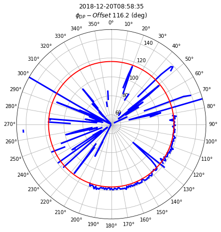
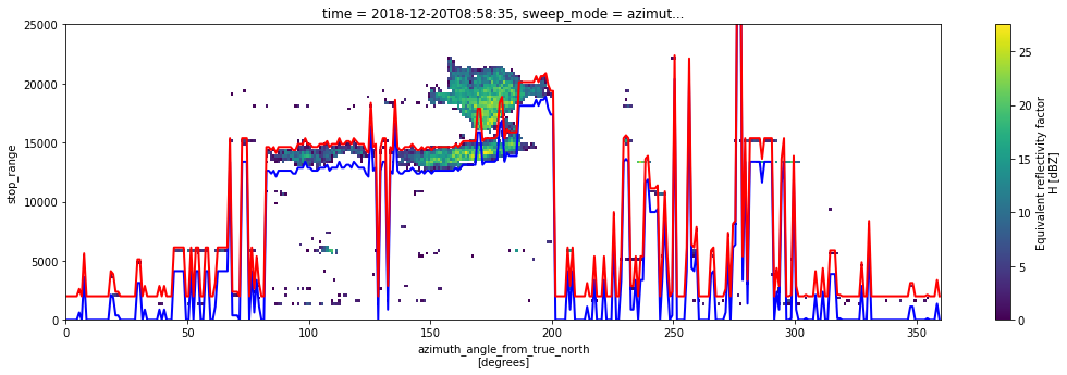
fig = plt.figure(figsize=(18, 5))
swp_msk.DBZH.plot(x="azimuth")
off.start_range.plot(c="b", lw=2)
off.stop_range.plot(c="r", lw=2)
plt.gca().set_ylim(0, 25000)
(0.0, 25000.0)
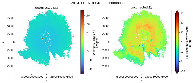
Process BoXPol data
vol = wrl.io.open_gamic_dataset(boxpol)
display(vol)
<wradlib.RadarVolume>
Dimension(s): (sweep: 1)
Elevation(s): (1.5)
swp = vol[0].copy()
swp = swp.pipe(wrl.georef.georeference_dataset)
display(swp)
<xarray.Dataset>
Dimensions:     (azimuth: 360, range: 1000)
Coordinates: (12/15)
  * azimuth     (azimuth) float64 0.5 1.5 2.5 3.5 ... 356.5 357.5 358.5 359.5
  * range       (range) float32 50.0 150.0 250.0 ... 9.985e+04 9.995e+04
    elevation   (azimuth) float64 1.505 1.505 1.505 1.505 ... 1.505 1.505 1.505
    rtime       (azimuth) datetime64[ns] 2014-11-16T03:48:49 ... 2014-11-16T0...
    time        datetime64[ns] 2014-11-16T03:48:38
    sweep_mode  <U20 'azimuth_surveillance'
    ...          ...
    x           (azimuth, range) float64 0.4362 1.309 2.181 ... -870.7 -871.6
    y           (azimuth, range) float64 49.98 149.9 ... 9.978e+04 9.988e+04
    z           (azimuth, range) float64 100.9 103.5 ... 3.309e+03 3.313e+03
    gr          (azimuth, range) float64 49.98 149.9 ... 9.978e+04 9.988e+04
    rays        (azimuth, range) float64 0.5 0.5 0.5 0.5 ... 359.5 359.5 359.5
    bins        (azimuth, range) float32 50.0 150.0 ... 9.985e+04 9.995e+04
Data variables:
    KDP         (azimuth, range) float32 ...
    PHIDP       (azimuth, range) float32 ...
    DBZH        (azimuth, range) float32 ...
    DBZV        (azimuth, range) float32 ...
    RHOHV       (azimuth, range) float32 ...
    DBTH        (azimuth, range) float32 ...
    DBTV        (azimuth, range) float32 ...
    VRADH       (azimuth, range) float32 ...
    VRADV       (azimuth, range) float32 ...
    WRADH       (azimuth, range) float32 ...
    WRADV       (azimuth, range) float32 ...
    ZDR         (azimuth, range) float32 ...
Attributes: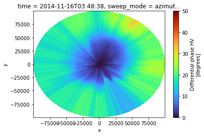
fixed_angle: 1.5Create Plot
fig = plt.figure(figsize=(13, 5))

ax1 = fig.add_subplot(121)
im1 = swp.PHIDP.where(swp.RHOHV > 0.8).plot(x="x", y="y", ax=ax1, cmap="turbo")
t = plt.title(r"Uncorrected $\phi_{DP}$")
t.set_y(1.1)

ax2 = fig.add_subplot(122)
im2 = swp.DBZH.where(swp.RHOHV > 0.8).plot(
    x="x", y="y", ax=ax2, cmap="turbo", vmin=-10, vmax=50
)
t = plt.title(r"Uncorrected $Z_{H}$")
t.set_y(1.1)
fig.suptitle(swp.time.values, fontsize=14)
fig.subplots_adjust(wspace=0.25)
Apply reasonable masking
dr_m = swp.range.diff("range").median()
swp_msk = swp.where((swp.DBZH >= 0.0))
swp_msk = swp_msk.where(swp_msk.RHOHV > 0.8)
swp_msk = swp_msk.where(swp_msk.range > dr_m * 2)


phi_masked = swp_msk.PHIDP.copy()
off = phase_offset(
    phi_masked, method="median", rng=2000.0, npix=7, center=True, min_periods=2
)
phioff = off.PHIDP_OFFSET.median(dim="azimuth", skipna=True)
Plot phase offset distribution
fig = plt.figure(figsize=(16, 7))
ax1 = plt.subplot(111, projection="polar")
# set the lable go clockwise and start from the top
ax1.set_theta_zero_location("N")
# clockwise
ax1.set_theta_direction(-1)
theta = np.linspace(0, 2 * np.pi, num=360, endpoint=False)
ax1.plot(theta, off.PHIDP_OFFSET, color="b", linewidth=3)

ax1.plot(theta, np.ones_like(theta) * phioff.values, color="r", lw=2)
ti = off.time.values.astype("M8[s]")
om = phioff.values
tx = ax1.set_title(f"{ti}\n" + r"$\phi_{DP}-Offset$ " + f"{om:.1f} (deg)")
tx.set_y(1.1)
xticks = ax1.set_xticks(np.pi / 180.0 * np.linspace(0, 360, 36, endpoint=False))
ax1.set_ylim(-120, -70)
(-120.0, -70.0)
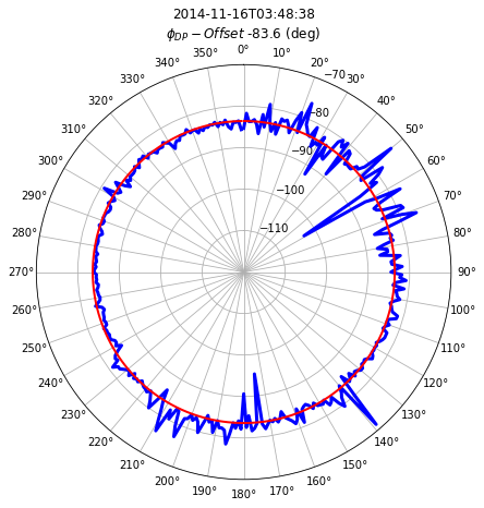
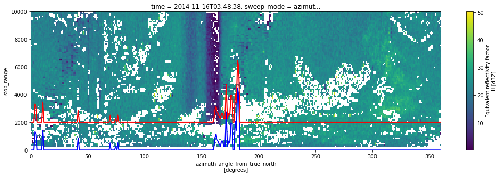
fig = plt.figure(figsize=(18, 5))
swp_msk.DBZH.plot(x="azimuth")
off.start_range.plot(c="b", lw=2)
off.stop_range.plot(c="r", lw=2)
plt.gca().set_ylim(0, 10000)
(0.0, 10000.0)
Pleaser refer to the ZPHI-Method section at the bottom of this notebook for references and equations.
Retrieving \(\Delta \phi_{DP}\)
We will use the simple method of finding the first and the last non NAN values per ray from \(\phi_{DP}^{corr}\).
This is the most simple and probably not very robust method.
def phase_zphi(phi, rng=1000.0, **kwargs):
    range_step = np.diff(phi.range)[0]

    nprec = int(rng / range_step)

    if nprec % 2:
        nprec += 1

    # create binary array
    phib = xr.where(np.isnan(phi), 0, 1)

    # take nprec range bins and calculate sum
    phib_sum = phib.rolling(range=nprec, **kwargs).sum(skipna=True)

    offset = nprec // 2 * np.diff(phib_sum.range)[0]
    offset_idx = nprec // 2

    start_range = phib_sum.idxmax(dim="range") - offset
    start_range_idx = phib_sum.argmax(dim="range") - offset_idx

    stop_range = phib_sum[:, ::-1].idxmax(dim="range") - offset
    stop_range_idx = (
        len(phib_sum.range) - (phib_sum[:, ::-1].argmax(dim="range") - offset_idx) - 2
    )

    # get phase values in specified range
    first = phi.where(
        (phi.range >= start_range) & (phi.range <= start_range + rng), drop=True
    ).quantile(0.15, dim="range", skipna=True)
    last = phi.where(
        (phi.range >= stop_range - rng) & (phi.range <= stop_range), drop=True
    ).quantile(0.95, dim="range", skipna=True)

    return xr.Dataset(
        dict(
            phib=phib_sum,
            offset=offset,
            offset_idx=offset_idx,
            start_range=start_range,
            stop_range=stop_range,
            first=first.drop("quantile"),
            first_idx=start_range_idx,
            last=last.drop("quantile"),
            last_idx=stop_range_idx,
        )
    )
Apply extraction of phase parameters.
cphase = phase_zphi(swp_msk.PHIDP, rng=2000.0, center=True, min_periods=7)
Apply azimuthal averaging.
cphase = (
    cphase.pad(pad_width={"azimuth": 2}, mode="wrap")
    .rolling(azimuth=5, center=True)
    .median(skipna=True)
    .isel(azimuth=slice(2, -2))
)
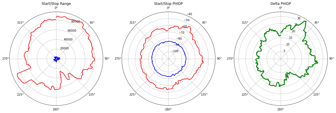
\(\Delta \phi_{DP}\) - Polar Plots
This visualizes first and last indizes including \(\Delta \phi_{DP}\).
dphi = cphase.last - cphase.first
dphi = dphi.where(dphi >= 0).fillna(0)
fig = plt.figure(figsize=(20, 9))
ax1 = plt.subplot(131, projection="polar")
ax2 = plt.subplot(132, projection="polar")
ax3 = plt.subplot(133, projection="polar")
# set the lable go clockwise and start from the top
ax1.set_theta_zero_location("N")
ax2.set_theta_zero_location("N")
ax3.set_theta_zero_location("N")
# clockwise
ax1.set_theta_direction(-1)
ax2.set_theta_direction(-1)
ax3.set_theta_direction(-1)
theta = np.linspace(0, 2 * np.pi, num=360, endpoint=False)
ax1.plot(theta, cphase.start_range, color="b", linewidth=2)
ax1.plot(theta, cphase.stop_range, color="r", linewidth=2)
_ = ax1.set_title("Start/Stop Range")

ax2.plot(theta, cphase.first, color="b", linewidth=2)
ax2.plot(theta, cphase.last, color="r", linewidth=2)
_ = ax2.set_title("Start/Stop PHIDP")
ax2.set_ylim(-110, -40)

ax3.plot(theta, dphi, color="g", linewidth=3)
# ax3.plot(theta, dphi_old, color="k", linewidth=1)
_ = ax3.set_title("Delta PHIDP")
Calculating \(f\Delta\phi_{DP}\)
# todo: cband coeffizienten
alphax = 0.28
betax = 0.05
bx = 0.78
# need to expand alphax to dphi-shape
fdphi = 10 ** (0.1 * bx * alphax * dphi) - 1
fdphi
<xarray.DataArray (azimuth: 360)>
array([1.50772944, 1.621746  , 1.63263211, 1.59938947, 1.77879842,
       1.87674877, 1.91353846, 1.96305219, 1.96305219, 1.97124872,
       2.29083108, 2.25196971, 2.31872025, 2.39724185, 2.37292792,
       2.49336399, 2.49336399, 2.4702802 , 2.05962546, 2.05962546,
       1.98779264, 2.08415043, 2.22085707, 2.33125884, 2.6826384 ,
       2.81518698, 2.85859008, 2.86824995, 2.85859008, 3.03636579,
       3.18973989, 3.43876111, 3.89274439, 3.89274439, 4.04998114,
       3.7410609 , 3.5279313 , 3.29545116, 3.13226527, 2.63714176,
       2.68060436, 2.68060436, 2.63714176, 2.6171011 , 2.68569016,
       2.42366977, 2.41700817, 2.38506371, 2.17667475, 2.11841838,
       1.87436571, 1.71911294, 1.76150461, 1.87436571, 2.01607107,
       2.01607107, 2.04992121, 2.0311066 , 2.01923888, 1.77006176,
       1.88550466, 1.85852905, 1.88630187, 1.93616259, 1.94184574,
       1.94184574, 1.88550356, 1.88494586, 1.87801993, 1.87801993,
       1.98605966, 1.96387083, 1.98770987, 2.13569607, 2.00903912,
       2.00903912, 2.06478535, 2.02759084, 1.92099396, 1.90831172,
       1.87333389, 1.8936456 , 1.8936456 , 2.05362955, 2.0340373 ,
       2.36548218, 2.40602815, 2.40602815, 2.39442893, 2.43024869,
       2.40475917, 2.35513227, 2.38211962, 2.38960217, 2.68670986,
       2.4064985 , 2.76909239, 2.76909239, 2.44544354, 2.39161573,
...
       1.48493842, 1.40258469, 1.35526881, 1.35526881, 1.36570186,
       1.36570186, 1.41723047, 1.45288304, 1.43734691, 1.43734691,
       1.3127157 , 1.18417608, 1.20235217, 1.17394212, 1.17394212,
       1.27155794, 1.1853823 , 1.30506194, 1.35140081, 1.39781004,
       1.4092306 , 1.42928047, 1.41776486, 1.40155549, 1.43562991,
       1.3748696 , 1.41656282, 1.3748696 , 1.3429393 , 1.31783232,
       1.19242757, 1.14515811, 1.13333828, 1.12173051, 1.14116148,
       1.14836012, 1.21945297, 1.22129306, 1.3589155 , 1.34099845,
       1.32938614, 1.38209702, 1.34488177, 1.28477377, 1.27847183,
       1.32231864, 1.39661884, 1.47261211, 1.47261211, 1.40856539,
       1.45742654, 1.4808222 , 1.64794967, 1.53695988, 1.51025952,
       1.38473063, 1.38078131, 1.37093571, 1.34734462, 1.30716441,
       1.26344584, 1.34410378, 1.34734462, 1.39605621, 1.67293704,
       1.77450348, 1.81270428, 1.91514859, 1.84828094, 1.93210992,
       1.83807067, 1.93210992, 1.94916881, 1.97239827, 1.91192921,
       1.93486535, 1.91192921, 1.94949493, 1.91353846, 2.13396412,
       2.1055235 , 1.96059651, 1.86960552, 1.96059651, 1.89748485,
       1.80843354, 1.85056417, 1.74022627, 1.80525399, 1.80215598,
       1.66482719, 1.64868023, 1.62798185, 1.45695102, 1.47261211,
       1.28540588, 1.26341505, 1.26341505, 1.30888565, 1.28414358])
Coordinates:
  * azimuth     (azimuth) float64 0.5 1.5 2.5 3.5 ... 356.5 357.5 358.5 359.5
    elevation   (azimuth) float64 1.505 1.505 1.505 1.505 ... 1.505 1.505 1.505
    rtime       (azimuth) datetime64[ns] 2014-11-16T03:48:49 ... 2014-11-16T0...
    time        datetime64[ns] 2014-11-16T03:48:38
    sweep_mode  <U20 'azimuth_surveillance'
    longitude   float64 7.072
    latitude    float64 50.73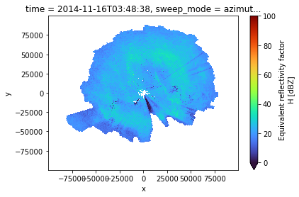
altitude float64 99.5Calculating Reflectivity Integrals/Sums
We do not restrict (mask) the reflectivities for now, but switch between DBTH and DBZH to see the difference.
zhraw = swp.DBZH.where(
    (swp.range > cphase.start_range) & (swp.range < cphase.stop_range)
)
zhraw.plot(x="x", y="y", cmap="turbo", vmin=0, vmax=100)
<matplotlib.collections.QuadMesh at 0x7f3ed00b8340>
# calculate linear reflectivity and ^b
zax = zhraw.pipe(wrl.trafo.idecibel).fillna(0)
za = zax**bx
# set masked to zero for integration
za_zero = za.fillna(0)
Calculate cumulative integral, and subtract from maximum. That way we have the cumulative sum for every bin until the end of the ray.
def cumulative_trapezoid_xarray(da, dim, initial=0):
    """Intgration with the scipy.integrate.cumtrapz.

    Parameter
    ---------
    da : xarray.DataArray
        array with differential phase data
    dim : int
        size of window in range dimension

    Keyword Arguments
    -----------------
    initial : float
        minimum number of valid bins

    Return
    ------
    kdp : xarray.DataArray
        DataArray with specific differential phase values
    """
    x = da[dim]
    dx = x.diff(dim).median(dim).values
    if x.attrs["units"] == "meters":
        dx /= 1000.0
    return xr.apply_ufunc(
        cumulative_trapezoid,
        da,
        input_core_dims=[[dim]],
        output_core_dims=[[dim]],
        dask="parallelized",
        kwargs=dict(axis=da.get_axis_num(dim), initial=initial, dx=dx),
        dask_gufunc_kwargs=dict(allow_rechunk=True),
    )
iza_x = 0.46 * bx * za_zero.pipe(cumulative_trapezoid_xarray, "range", initial=0)
iza = iza_x.max("range") - iza_x
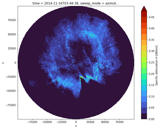
Calculating Attenuation \(A_{H}\) for whole domain
We can reduce the number of operations by rearranging the equation like this:
iza_fdphi = iza / fdphi
idx = cphase.first_idx.astype(int)
iza_first = iza_fdphi[:, idx]
ah = za / (iza_first + iza)
Give it a name!
ah.name = "AH"
ah.attrs["short_name"] = "specific_attenuation_h"
ah.attrs["long_name"] = "Specific attenuation H"
ah.attrs["units"] = "dB/km"
fig = plt.figure(figsize=(10, 8))
ax = fig.add_subplot(111)
ticks_ah = np.arange(0, 5, 0.2)
im = ah.plot(x="x", y="y", ax=ax, cmap="turbo", levels=np.arange(0, 0.5, 0.025))
Calculate \(\phi_{DP}^{cal}(r, \alpha)\) for whole domain
phical = 2 * (ah / alphax).pipe(cumulative_trapezoid_xarray, "range", initial=0)
phical.name = "PHICAL"
phical.attrs = wrl.io.xarray.moments_mapping["PHIDP"]
phical.where(swp_msk.PHIDP).plot(x="x", y="y", vmin=0, vmax=50, cmap="turbo")
<matplotlib.collections.QuadMesh at 0x7f3ec9f24c40>
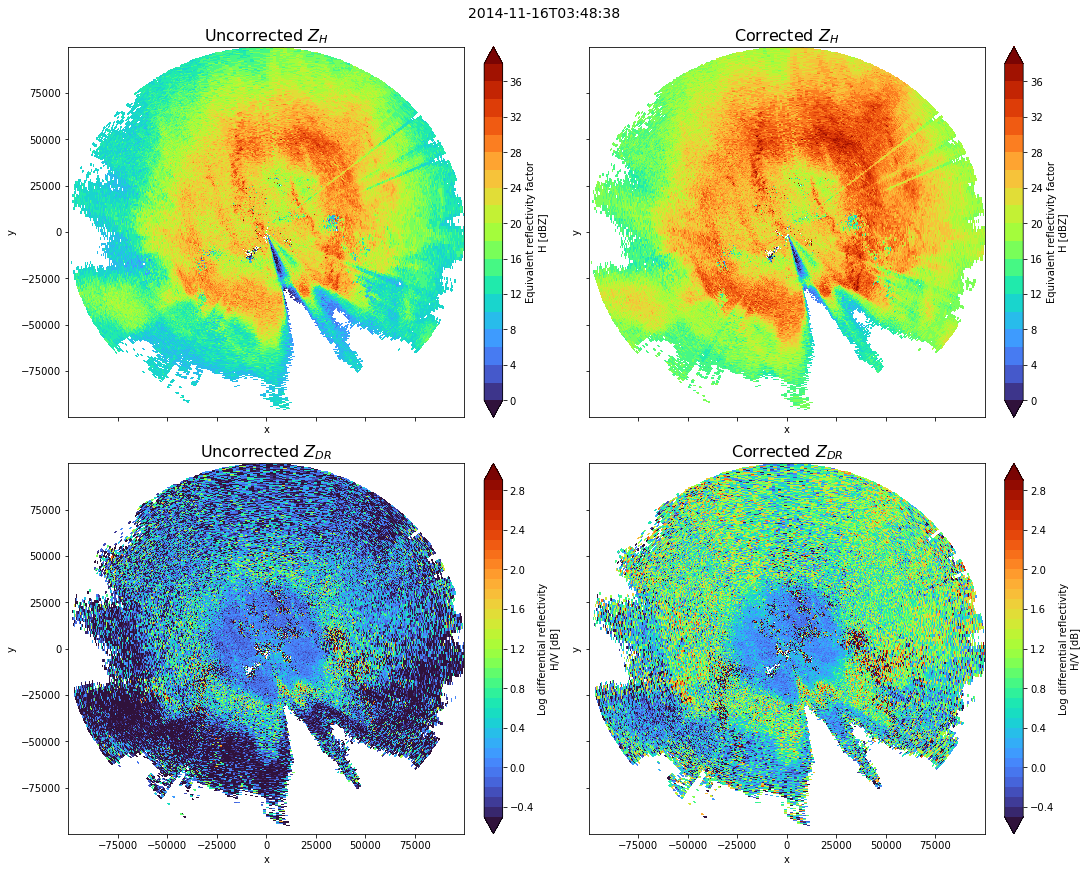
Apply attenuation correction
print(alphax)
0.28
zhraw = swp.DBZH.copy()
zdrraw = swp.ZDR.copy()
with xr.set_options(keep_attrs=True):
    zhcorr = zhraw + alphax * (phical)
    zdiff = zhcorr - zhraw
    zdrcorr = zdrraw + betax * (phical)
    zdrdiff = zdrcorr - zdrraw
fig, ((ax1, ax2), (ax3, ax4)) = plt.subplots(
    nrows=2,
    ncols=2,
    figsize=(15, 12),
    sharex=True,
    sharey=True,
    squeeze=True,
    constrained_layout=True,
)

scantime = zhraw.time.values.astype("<M8[s]")
t = fig.suptitle(scantime, fontsize=14)
t.set_y(1.05)

zhraw.plot(x="x", y="y", ax=ax1, cmap="turbo", levels=np.arange(0, 40, 2))
ax1.set_title(r"Uncorrected $Z_{H}$", fontsize=16)
zhcorr.plot(x="x", y="y", ax=ax2, cmap="turbo", levels=np.arange(0, 40, 2))
ax2.set_title(r"Corrected $Z_{H}$", fontsize=16)

zdrraw.plot(x="x", y="y", ax=ax3, cmap="turbo", levels=np.arange(-0.5, 3, 0.1))
ax3.set_title(r"Uncorrected $Z_{DR}$", fontsize=16)
zdrcorr.plot(x="x", y="y", ax=ax4, cmap="turbo", levels=np.arange(-0.5, 3, 0.1))
ax4.set_title(r"Corrected $Z_{DR}$", fontsize=16)
Text(0.5, 1.0, 'Corrected $Z_{DR}$')
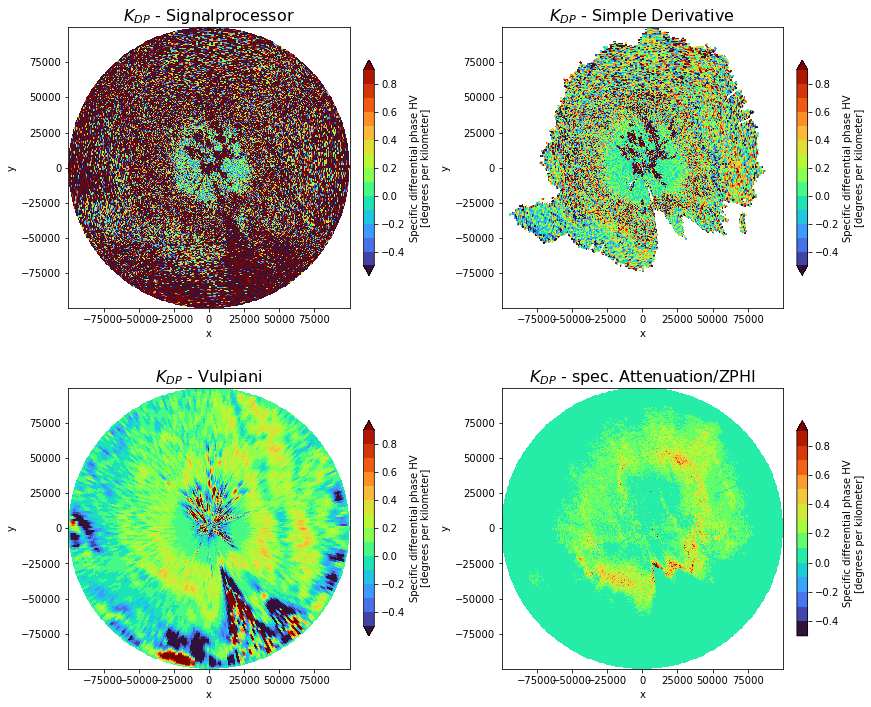
\(K_{DP}\) from \(A_H\) vs. \(K_{DP}\) from \(\phi_{DP}\)
\(K_{DP} = \frac{A_H}{\alpha}\)
\(K_{DP} = \frac{1}{2}\frac{\mathrm{d}\phi_{DP}}{\mathrm{d}r}\)
What are the benefits of \(K_{DP}(A_H)\)?
no noise artefacts
no \(\delta\)
no negative \(K_{DP}\)
no spatial degradation
def kdp_from_phidp(da, winlen, min_periods=2):
    """Derive KDP from PHIDP (based on convolution filter).

    Parameter
    ---------
    da : xarray.DataArray
        array with differential phase data
    winlen : int
        size of window in range dimension

    Keyword Arguments
    -----------------
    min_periods : int
        minimum number of valid bins

    Return
    ------
    kdp : xarray.DataArray
        DataArray with specific differential phase values
    """
    dr = da.range.diff("range").median("range").values / 1000.0
    print("range res [km]:", dr)
    print("processing window [km]:", dr * winlen)
    return xr.apply_ufunc(
        wrl.dp.kdp_from_phidp,
        da,
        input_core_dims=[["range"]],
        output_core_dims=[["range"]],
        dask="parallelized",
        kwargs=dict(winlen=winlen, dr=dr, min_periods=min_periods),
        dask_gufunc_kwargs=dict(allow_rechunk=True),
    )


def kdp_phidp_vulpiani(da, winlen, min_periods=2):
    """Derive KDP from PHIDP (based on Vulpiani).

    ParameterRHOHV_NC
    ---------
    da : xarray.DataArray
        array with differential phase data
    winlen : int
        size of window in range dimension

    Keyword Arguments
    -----------------
    min_periods : int
        minimum number of valid bins

    Return
    ------
    kdp : xarray.DataArray
        DataArray with specific differential phase values
    """
    dr = da.range.diff("range").median("range").values / 1000.0
    print("range res [km]:", dr)
    print("processing window [km]:", dr * winlen)
    return xr.apply_ufunc(
        wrl.dp.process_raw_phidp_vulpiani,
        da,
        input_core_dims=[["range"]],
        output_core_dims=[["range"], ["range"]],
        dask="parallelized",
        kwargs=dict(winlen=winlen, dr=dr, min_periods=min_periods),
        dask_gufunc_kwargs=dict(allow_rechunk=True),
    )
%%time
kdp1 = kdp_from_phidp(swp_msk.PHIDP, winlen=31, min_periods=11)
kdp1.attrs = wrl.io.xarray.moments_mapping["KDP"]

kdp2 = kdp_phidp_vulpiani(swp.PHIDP, winlen=71, min_periods=21)[1]
kdp2.attrs = wrl.io.xarray.moments_mapping["KDP"]

kdp3 = xr.zeros_like(kdp1)
kdp3.attrs = wrl.io.xarray.moments_mapping["KDP"]
kdp3.data = ah / alphax
range res [km]: 0.1
processing window [km]: 3.1
range res [km]: 0.1
processing window [km]: 7.1000000000000005
CPU times: user 341 ms, sys: 44 ms, total: 385 ms
Wall time: 383 ms
fig, ((ax1, ax2), (ax3, ax4)) = plt.subplots(
    nrows=2, ncols=2, figsize=(12, 10), constrained_layout=True
)

swp.KDP.plot(
    x="x",
    y="y",
    ax=ax1,
    cmap="turbo",
    levels=np.arange(-0.5, 1, 0.1),
    cbar_kwargs=dict(shrink=0.64),
)
ax1.set_title(r"$K_{DP}$ - Signalprocessor", fontsize=16)
ax1.set_aspect("equal")
kdp1.plot(
    x="x",
    y="y",
    ax=ax2,
    cmap="turbo",
    levels=np.arange(-0.5, 1, 0.1),
    cbar_kwargs=dict(shrink=0.64),
)
ax2.set_title(r"$K_{DP}$ - Simple Derivative", fontsize=16)
ax2.set_aspect("equal")
kdp2.plot(
    x="x",
    y="y",
    ax=ax3,
    cmap="turbo",
    levels=np.arange(-0.5, 1, 0.1),
    cbar_kwargs=dict(shrink=0.64),
)
ax3.set_title(r"$K_{DP}$ - Vulpiani", fontsize=16)
ax3.set_aspect("equal")
kdp3.plot(
    x="x",
    y="y",
    ax=ax4,
    cmap="turbo",
    levels=np.arange(-0.5, 1, 0.1),
    cbar_kwargs=dict(shrink=0.64),
)
ax4.set_title(r"$K_{DP}$ - spec. Attenuation/ZPHI", fontsize=16)
ax4.set_aspect("equal")
Summary
We’ve just learned how to derive System Phase Offset and Specific Attenuation AH using the ZPHI-Method. Different KDP derivation methods have been compared.
Resources and references
Testud, J., Le Bouar, E., Obligis, E., & Ali-Mehenni, M. (2000). The Rain Profiling Algorithm Applied to Polarimetric Weather Radar, Journal of Atmospheric and Oceanic Technology, 17(3), 332-356. Retrieved Nov 24, 2021, from https://journals.ametsoc.org/view/journals/atot/17/3/1520-0426_2000_017_0332_trpaat_2_0_co_2.xml
Diederich, M., Ryzhkov, A., Simmer, C., Zhang, P., & Trömel, S. (2015). Use of Specific Attenuation for Rainfall Measurement at X-Band Radar Wavelengths.: Part I: Radar Calibration and Partial Beam Blockage Estimation. Journal of Hydrometeorology, 16(2), 487–502. http://www.jstor.org/stable/24914953
ZPHI-Method
see Testud et.al. (chapter 4. p. 339ff.), Diederich et.al. (chapter 3. p. 492 ff).
There is a equational difference in the two papers, which can be solved like this:
\(\begin{equation} f\Delta\phi_{DP} = 10^{0.1 \cdot b \cdot \alpha \cdot \Delta\phi_{DP}} - 1 \tag{1} \end{equation}\)
\(\begin{equation} C(b, PIA) = \exp[{0.23 \cdot b \cdot (PIA)}] - 1 \tag{2} \end{equation}\)
with
\(\begin{equation} PIA = \alpha \cdot \Delta\phi_{DP} \tag{3} \end{equation}\)
\(\begin{equation} C(b, PIA) = \exp[{0.23 \cdot b \cdot \alpha \cdot \Delta\phi_{DP}}] - 1 \tag{4} \end{equation}\)
Both expressions are used equivalently:
\(\begin{equation} 10^{0.1 \cdot b \cdot \alpha \cdot \Delta\phi_{DP}} - 1 = \exp[{0.23 \cdot b \cdot \alpha \cdot \Delta\phi_{DP}}] - 1 \tag{5} \end{equation}\)
Using logarithmic identities:
\(\begin{equation} \ln {u^r} = r \cdot \ln {u} \tag{6a} \end{equation}\)
\(\begin{equation} \exp {\ln x} = x \tag{6b} \end{equation}\)
the left hand side can be further expressed as:
\(\begin{equation} \exp [\ln {10^{0.1 \cdot b \cdot \alpha \cdot \Delta\phi_{DP}}}] - 1 = \exp[{0.23 \cdot b \cdot \alpha \cdot \Delta\phi_{DP}}] - 1 \tag{7a} \end{equation}\)
\(\begin{equation} \exp[0.1 \cdot b \cdot \alpha \cdot \Delta\phi_{DP} \cdot \ln {10}] - 1 = \exp[{0.23 \cdot b \cdot \alpha \cdot \Delta\phi_{DP}}] - 1 \tag{7b} \end{equation}\)
leading to equality
\(\begin{equation} \exp[0.23 \cdot b \cdot \alpha \cdot \Delta\phi_{DP}] - 1 = \exp[{0.23 \cdot b \cdot \alpha \cdot \Delta\phi_{DP}}] - 1 \tag{7c} \end{equation}\)