.ipynb .pdf

repository open issue suggest edit

On this page

wradlib radar data io, visualisation, gridding and gis export

---

Overview

Within this notebook, we will cover:

1. Reading radar volume data into xarray based RadarVolume

2. Examination of RadarVolume and Sweeps

3. Plotting of sweeps, simple and mapmaking

4. Gridding and GIS output

Prerequisites

Concepts	Importance	Notes
Xarray Basics	Helpful	Basic Dataset/DataArray
Matplotlib Basics	Helpful	Basic Plotting
Cartopy Basics	Helpful	Projections
GDAL Basiscs	Helpful	Raster

• Time to learn: 15 minutes

---

Imports

import glob
import pathlib

import cartopy
import cartopy.crs as ccrs
import cartopy.feature as cfeature
import matplotlib.pyplot as plt
import numpy as np
import xarray as xr
from matplotlib import ticker as tick
from osgeo import gdal

import wradlib as wrl

/srv/conda/envs/notebook/lib/python3.9/site-packages/requests/__init__.py:102: RequestsDependencyWarning: urllib3 (1.26.8) or chardet (5.2.0)/charset_normalizer (2.0.10) doesn't match a supported version!
  warnings.warn("urllib3 ({}) or chardet ({})/charset_normalizer ({}) doesn't match a supported "

Import data into RadarVolume

We have this special case here with Rainbow data where moments are splitted across files. Each file nevertheless consists of all sweeps comprising the volume. We’ll use some special nested ordering to read the files.

fglob = "data/rainbow/meteoswiss/*.vol"

vol = wrl.io.open_rainbow_mfdataset(fglob, combine="by_coords", concat_dim=None)

Examine RadarVolume

The RadarVolume is a shallow class which tries to comply to CfRadial2/WMO-FM301, see WMO-CF_Extensions.

The printout of RadarVolume just lists the dimensions and the associated elevations.

display(vol)

<wradlib.RadarVolume>
Dimension(s): (sweep: 10)
Elevation(s): (0.0, 1.3, 2.9, 4.9, 7.3, 10.2, 13.8, 18.2, 23.5, 30.0)

Root Group

The root-group is essentially an overview over the volume, more or less aligned with CfRadial metadata.

vol.root

<xarray.Dataset>
Dimensions:              (sweep: 10)
Coordinates:
    time                 datetime64[ns] 2019-10-21T08:24:09
    longitude            float64 6.954
    altitude             float64 735.0
    sweep_mode           <U20 'azimuth_surveillance'
    latitude             float64 46.77
Dimensions without coordinates: sweep
Data variables:
    volume_number        int64 0
    platform_type        <U5 'fixed'
    instrument_type      <U5 'radar'
    primary_axis         <U6 'axis_z'
    time_coverage_start  <U20 '2019-10-21T08:24:09Z'
    time_coverage_end    <U20 '2019-10-21T08:29:33Z'
    sweep_group_name     (sweep) <U7 'sweep_0' 'sweep_1' ... 'sweep_8' 'sweep_9'
    sweep_fixed_angle    (sweep) float64 0.0 1.3 2.9 4.9 ... 13.8 18.2 23.5 30.0
Attributes:
    version:          None
    title:            None
    institution:      None
    references:       None
    source:           None
    history:          None
    comment:          im/exported using wradlib
    instrument_name:  None
    fixed_angle:      0.0

xarray.Dataset

• Dimensions:
  • sweep: 10
• Coordinates: (5)
  • time
    ()
    datetime64[ns]
    2019-10-21T08:24:09

    standard_name :

    time

    array('2019-10-21T08:24:09.000000000', dtype='datetime64[ns]')

  • longitude
    ()
    float64
    6.954

    long_name :

    longitude

    units :

    degrees_east

    standard_name :

    longitude

    array(6.953958)

  • altitude
    ()
    float64
    735.0

    long_name :

    altitude

    units :

    meters

    standard_name :

    altitude

    array(735.)

  • sweep_mode
    ()
    <U20
    'azimuth_surveillance'

    array('azimuth_surveillance', dtype='<U20')

  • latitude
    ()
    float64
    46.77

    long_name :

    latitude

    units :

    degrees_north

    positive :

    up

    standard_name :

    latitude

    array(46.769715)

• Data variables: (8)
  • volume_number
    ()
    int64
    0

    array(0)

  • platform_type
    ()
    <U5
    'fixed'

    array('fixed', dtype='<U5')

  • instrument_type
    ()
    <U5
    'radar'

    array('radar', dtype='<U5')

  • primary_axis
    ()
    <U6
    'axis_z'

    array('axis_z', dtype='<U6')

  • time_coverage_start
    ()
    <U20
    '2019-10-21T08:24:09Z'

    array('2019-10-21T08:24:09Z', dtype='<U20')

  • time_coverage_end
    ()
    <U20
    '2019-10-21T08:29:33Z'

    array('2019-10-21T08:29:33Z', dtype='<U20')

  • sweep_group_name
    (sweep)
    <U7
    'sweep_0' 'sweep_1' ... 'sweep_9'

    array(['sweep_0', 'sweep_1', 'sweep_2', 'sweep_3', 'sweep_4', 'sweep_5',
           'sweep_6', 'sweep_7', 'sweep_8', 'sweep_9'], dtype='<U7')

  • sweep_fixed_angle
    (sweep)
    float64
    0.0 1.3 2.9 4.9 ... 18.2 23.5 30.0

    array([ 0. ,  1.3,  2.9,  4.9,  7.3, 10.2, 13.8, 18.2, 23.5, 30. ])

• Attributes: (9)

  version :

  None

  title :

  None

  institution :

  None

  references :

  None

  source :

  None

  history :

  None

  comment :

  im/exported using wradlib

  instrument_name :

  None

  fixed_angle :

  0.0

Sweep Groups

Sweeps are available in a sequence attached to the RadarVolume object.

swp = vol[0]
display(swp)

<xarray.Dataset>
Dimensions:     (azimuth: 360, range: 1400)
Coordinates:
  * azimuth     (azimuth) float64 0.5 1.5 2.5 3.5 ... 356.5 357.5 358.5 359.5
  * range       (range) float32 25.0 75.0 125.0 ... 6.992e+04 6.998e+04
    elevation   (azimuth) float64 dask.array<chunksize=(360,), meta=np.ndarray>
    time        datetime64[ns] 2019-10-21T08:24:09
    rtime       (azimuth) datetime64[ns] dask.array<chunksize=(360,), meta=np.ndarray>
    longitude   float64 6.954
    latitude    float64 46.77
    altitude    float64 735.0
    sweep_mode  <U20 'azimuth_surveillance'
Data variables:
    DBZH        (azimuth, range) float32 dask.array<chunksize=(360, 1400), meta=np.ndarray>
    KDP         (azimuth, range) float32 dask.array<chunksize=(360, 1400), meta=np.ndarray>
    PHIDP       (azimuth, range) float32 dask.array<chunksize=(360, 1400), meta=np.ndarray>
    RHOHV       (azimuth, range) float32 dask.array<chunksize=(360, 1400), meta=np.ndarray>
    VRADH       (azimuth, range) float32 dask.array<chunksize=(360, 1400), meta=np.ndarray>
    WRADH       (azimuth, range) float32 dask.array<chunksize=(360, 1400), meta=np.ndarray>
    ZDR         (azimuth, range) float32 dask.array<chunksize=(360, 1400), meta=np.ndarray>
Attributes: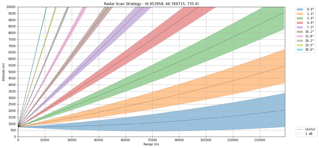
    fixed_angle:  0.0

xarray.Dataset

• Dimensions:
  • azimuth: 360
  • range: 1400
• Coordinates: (9)
  • azimuth
    (azimuth)
    float64
    0.5 1.5 2.5 ... 357.5 358.5 359.5

    standard_name :

    ray_azimuth_angle

    long_name :

    azimuth_angle_from_true_north

    units :

    degrees

    axis :

    radial_azimuth_coordinate

    a1gate :

    133

    angle_res :

    1.0

    array([  0.5,   1.5,   2.5, ..., 357.5, 358.5, 359.5])

  • range
    (range)
    float32
    25.0 75.0 ... 6.992e+04 6.998e+04

    units :

    meters

    standard_name :

    projection_range_coordinate

    long_name :

    range_to_measurement_volume

    spacing_is_constant :

    true

    axis :

    radial_range_coordinate

    meters_to_center_of_first_gate :

    25.0

    meters_between_gates :

    50.0

    array([2.5000e+01, 7.5000e+01, 1.2500e+02, ..., 6.9875e+04, 6.9925e+04,
           6.9975e+04], dtype=float32)

  • elevation
    (azimuth)
    float64
    dask.array<chunksize=(360,), meta=np.ndarray>

    standard_name :

    ray_elevation_angle

    long_name :

    elevation_angle_from_horizontal_plane

    units :

    degrees

    axis :

    radial_elevation_coordinate

    Array Chunk Bytes 2.81 kiB 2.81 kiB Shape (360,) (360,) Count 30 Graph Layers 1 Chunks Type float64 numpy.ndarray

  • time
    ()
    datetime64[ns]
    2019-10-21T08:24:09

    standard_name :

    time

    array('2019-10-21T08:24:09.000000000', dtype='datetime64[ns]')

  • rtime
    (azimuth)
    datetime64[ns]
    dask.array<chunksize=(360,), meta=np.ndarray>

    standard_name :

    time

    Array Chunk Bytes 2.81 kiB 2.81 kiB Shape (360,) (360,) Count 30 Graph Layers 1 Chunks Type datetime64[ns] numpy.ndarray

  • longitude
    ()
    float64
    6.954

    long_name :

    longitude

    units :

    degrees_east

    standard_name :

    longitude

    array(6.953958)

  • latitude
    ()
    float64
    46.77

    long_name :

    latitude

    units :

    degrees_north

    positive :

    up

    standard_name :

    latitude

    array(46.769715)

  • altitude
    ()
    float64
    735.0

    long_name :

    altitude

    units :

    meters

    standard_name :

    altitude

    array(735.)

  • sweep_mode
    ()
    <U20
    'azimuth_surveillance'

    array('azimuth_surveillance', dtype='<U20')

• Data variables: (7)
  • DBZH
    (azimuth, range)
    float32
    dask.array<chunksize=(360, 1400), meta=np.ndarray>

    long_name :

    Equivalent reflectivity factor H

    standard_name :

    radar_equivalent_reflectivity_factor_h

    units :

    dBZ

    Array Chunk Bytes 1.92 MiB 1.92 MiB Shape (360, 1400) (360, 1400) Count 2 Graph Layers 1 Chunks Type float32 numpy.ndarray

  • KDP
    (azimuth, range)
    float32
    dask.array<chunksize=(360, 1400), meta=np.ndarray>

    long_name :

    Specific differential phase HV

    standard_name :

    radar_specific_differential_phase_hv

    units :

    degrees per kilometer

    Array Chunk Bytes 1.92 MiB 1.92 MiB Shape (360, 1400) (360, 1400) Count 2 Graph Layers 1 Chunks Type float32 numpy.ndarray

  • PHIDP
    (azimuth, range)
    float32
    dask.array<chunksize=(360, 1400), meta=np.ndarray>

    long_name :

    Differential phase HV

    standard_name :

    radar_differential_phase_hv

    units :

    degrees

    Array Chunk Bytes 1.92 MiB 1.92 MiB Shape (360, 1400) (360, 1400) Count 2 Graph Layers 1 Chunks Type float32 numpy.ndarray

  • RHOHV
    (azimuth, range)
    float32
    dask.array<chunksize=(360, 1400), meta=np.ndarray>

    long_name :

    Correlation coefficient HV

    standard_name :

    radar_correlation_coefficient_hv

    units :

    unitless

    Array Chunk Bytes 1.92 MiB 1.92 MiB Shape (360, 1400) (360, 1400) Count 2 Graph Layers 1 Chunks Type float32 numpy.ndarray

  • VRADH
    (azimuth, range)
    float32
    dask.array<chunksize=(360, 1400), meta=np.ndarray>

    long_name :

    Radial velocity of scatterers away from instrument H

    standard_name :

    radial_velocity_of_scatterers_away_from_instrument_h

    units :

    meters per seconds

    Array Chunk Bytes 1.92 MiB 1.92 MiB Shape (360, 1400) (360, 1400) Count 2 Graph Layers 1 Chunks Type float32 numpy.ndarray

  • WRADH
    (azimuth, range)
    float32
    dask.array<chunksize=(360, 1400), meta=np.ndarray>

    long_name :

    Doppler spectrum width H

    standard_name :

    radar_doppler_spectrum_width_h

    units :

    meters per seconds

    Array Chunk Bytes 1.92 MiB 1.92 MiB Shape (360, 1400) (360, 1400) Count 2 Graph Layers 1 Chunks Type float32 numpy.ndarray

  • ZDR
    (azimuth, range)
    float32
    dask.array<chunksize=(360, 1400), meta=np.ndarray>

    long_name :

    Log differential reflectivity H/V

    standard_name :

    radar_differential_reflectivity_hv

    units :

    dB

    Array Chunk Bytes 1.92 MiB 1.92 MiB Shape (360, 1400) (360, 1400) Count 2 Graph Layers 1 Chunks Type float32 numpy.ndarray

• Attributes: (1)

  fixed_angle :

  0.0

Inspect Scan Strategy

Considering volume files it’s nice to have an overview over the scan strategy. We can choose some reasonable values for the layout.

nrays = 360
nbins = 150
range_res = 1000.0
ranges = np.arange(nbins) * range_res
elevs = vol.root.sweep_fixed_angle.values
sitecoords = (
    vol.root.longitude.values.item(),
    vol.root.latitude.values.item(),
    vol.root.altitude.values.item(),
)

beamwidth = 1.0

ax = wrl.vis.plot_scan_strategy(ranges, elevs, sitecoords)

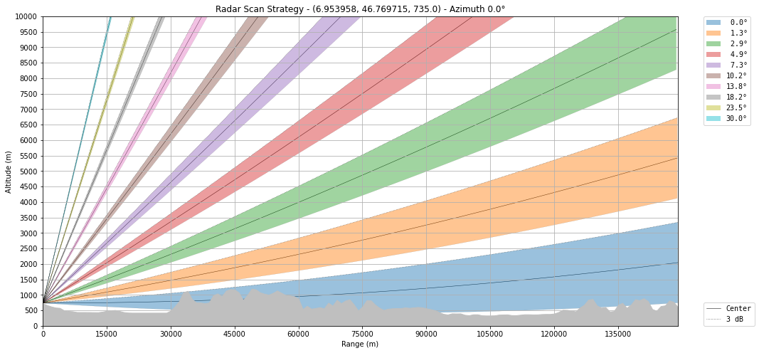
We can plot it on top of the terrain derived from SRTM DEM.

import os

os.environ["WRADLIB_EARTHDATA_BEARER_TOKEN"] = ""
os.environ["WRADLIB_DATA"] = "data/wradlib-data"

ax = wrl.vis.plot_scan_strategy(ranges, elevs, sitecoords, terrain=True)

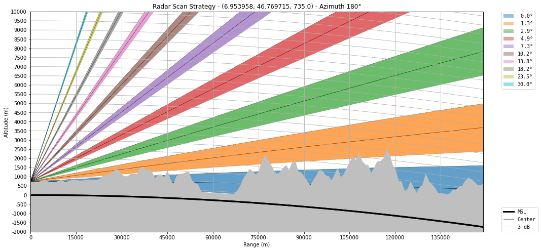
Let’s make the earth go round…

ax = wrl.vis.plot_scan_strategy(
    ranges, elevs, sitecoords, cg=True, terrain=True, az=180
)

Plotting Radar Data

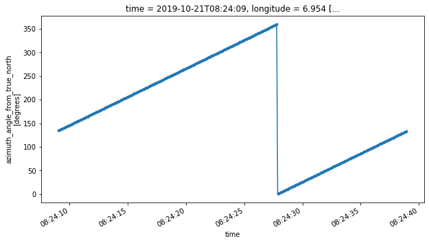
Time vs. Azimuth

fig = plt.figure(figsize=(10, 5))
ax1 = fig.add_subplot(111)
swp.azimuth.sortby("rtime").plot(x="rtime", marker=".")

[<matplotlib.lines.Line2D at 0x7fa684ced490>]

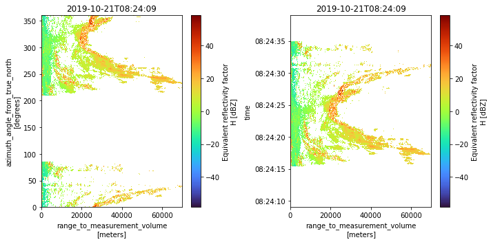
Range vs. Azimuth/Time

fig = plt.figure(figsize=(10, 5))
ax1 = fig.add_subplot(121)
swp.DBZH.plot(cmap="turbo", ax=ax1)
ax1.set_title(f"{swp.time.values.astype('M8[s]')}")
ax2 = fig.add_subplot(122)
swp.DBZH.sortby("rtime").plot(y="rtime", cmap="turbo", ax=ax2)
ax2.set_title(f"{swp.time.values.astype('M8[s]')}")
plt.tight_layout()

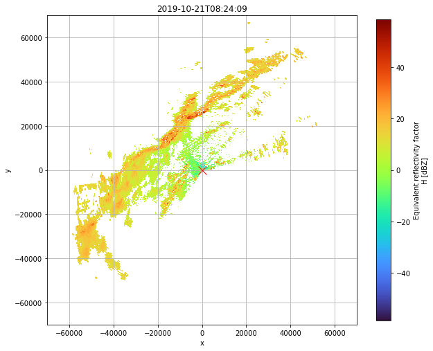
Georeferenced as Plan Position Indicator

fig = plt.figure(figsize=(10, 10))
ax1 = fig.add_subplot(111)
swp.DBZH.pipe(wrl.georef.georeference_dataset).plot(
    x="x", y="y", ax=ax1, cmap="turbo", cbar_kwargs=dict(shrink=0.8)
)
ax1.plot(0, 0, "rx", markersize=12)
ax1.set_title(f"{swp.time.values.astype('M8[s]')}")
ax1.grid()
ax1.set_aspect("equal")

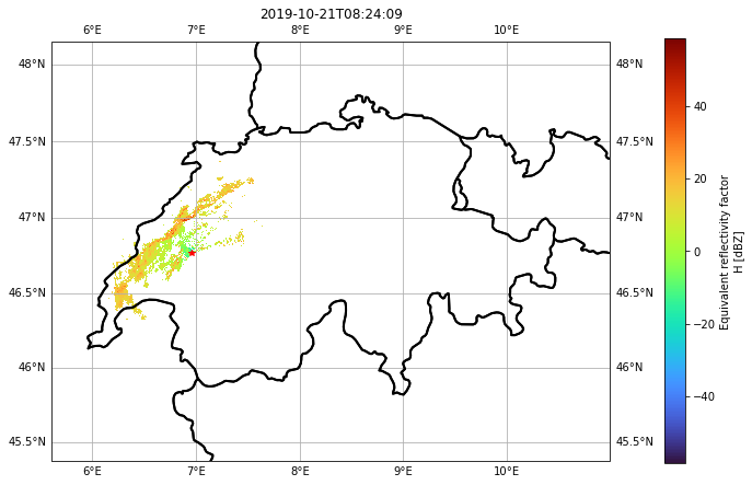
Basic MapMaking with cartopy

The data will be georeferenced as Azimuthal Equidistant Projection centered at the radar. For the map projection we will use Mercator.

map_trans = ccrs.AzimuthalEquidistant(
    central_latitude=swp.latitude.values, central_longitude=swp.longitude.values
)
map_proj = ccrs.Mercator(central_longitude=swp.longitude.values)

def plot_borders(ax):
    borders = cfeature.NaturalEarthFeature(
        category="cultural", name="admin_0_countries", scale="10m", facecolor="none"
    )
    ax.add_feature(borders, edgecolor="black", lw=2, zorder=4)

fig = plt.figure(figsize=(10, 8))
ax = fig.add_subplot(111, projection=map_proj)
cbar_kwargs = dict(shrink=0.7, pad=0.075)
pm = swp.DBZH.pipe(wrl.georef.georeference_dataset).plot(
    ax=ax, x="x", y="y", cbar_kwargs=cbar_kwargs, cmap="turbo", transform=map_trans
)
plot_borders(ax)
ax.gridlines(draw_labels=True)
ax.plot(
    swp.longitude.values, swp.latitude.values, transform=map_trans, marker="*", c="r"
)
ax.set_title(f"{swp.time.values.astype('M8[s]')}")
ax.set_xlim(-15e4, 45e4)
ax.set_ylim(565e4, 610e4)
plt.tight_layout()

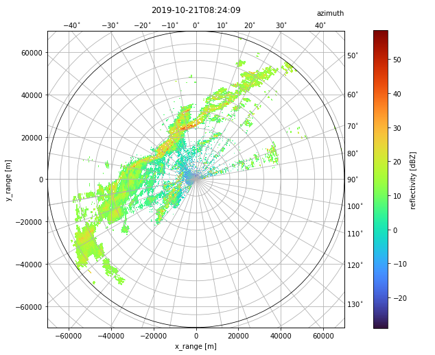
Plot on curvelinear grid

For Xarray DataArrays wradlib uses a so-called accessor (wradlib). To plot on curvelinear grids projection has to be set to cg, which uses the matplotlib AXISARTIS namespace.

fig = plt.figure(figsize=(10, 8))

pm = swp.DBZH.pipe(wrl.georef.georeference_dataset).wradlib.plot(
    proj="cg", fig=fig, cmap="turbo"
)

ax = plt.gca()

# apply eye-candy
caax = ax.parasites[0]
paax = ax.parasites[1]
ax.parasites[1].set_aspect("equal")
t = plt.title(f"{vol[0].time.values.astype('M8[s]')}", y=1.05)
cbar = plt.colorbar(pm, pad=0.075, ax=paax)
caax.set_xlabel("x_range [m]")
caax.set_ylabel("y_range [m]")
plt.text(1.0, 1.05, "azimuth", transform=caax.transAxes, va="bottom", ha="right")
cbar.set_label("reflectivity [dBZ]")

ODIM_H5 format export and import

Export to ODIM_H5

vol.to_odim("test_odim_vol.h5")

Import from ODIM_H5

vol2 = wrl.io.open_odim_dataset("test_odim_vol.h5")
display(vol2)

<wradlib.RadarVolume>
Dimension(s): (sweep: 10)
Elevation(s): (0.0, 1.3, 2.9, 4.9, 7.3, 10.2, 13.8, 18.2, 23.5, 30.0)

display(vol2[0])

<xarray.Dataset>
Dimensions:     (azimuth: 360, range: 1400)
Coordinates:
  * azimuth     (azimuth) float64 0.5 1.5 2.5 3.5 ... 356.5 357.5 358.5 359.5
    elevation   (azimuth) float64 0.0 0.0 0.0 0.0 0.0 ... 0.0 0.0 0.0 0.0 0.0
    rtime       (azimuth) datetime64[ns] 2019-10-21T08:24:27.875000064 ... 20...
  * range       (range) float32 25.0 75.0 125.0 ... 6.992e+04 6.998e+04
    time        datetime64[ns] 2019-10-21T08:24:09
    sweep_mode  <U20 'azimuth_surveillance'
    longitude   float64 6.954
    latitude    float64 46.77
    altitude    float64 735.0
Data variables:
    DBZH        (azimuth, range) float32 ...
    KDP         (azimuth, range) float32 ...
    PHIDP       (azimuth, range) float32 ...
    RHOHV       (azimuth, range) float32 ...
    VRADH       (azimuth, range) float32 ...
    WRADH       (azimuth, range) float32 ...
    ZDR         (azimuth, range) float32 ...
Attributes:
    fixed_angle:  0.0

xarray.Dataset

• Dimensions:
  • azimuth: 360
  • range: 1400
• Coordinates: (9)
  • azimuth
    (azimuth)
    float64
    0.5 1.5 2.5 ... 357.5 358.5 359.5

    standard_name :

    ray_azimuth_angle

    long_name :

    azimuth_angle_from_true_north

    units :

    degrees

    axis :

    radial_azimuth_coordinate

    a1gate :

    134

    angle_res :

    1.0

    array([  0.5,   1.5,   2.5, ..., 357.5, 358.5, 359.5])

  • elevation
    (azimuth)
    float64
    ...

    standard_name :

    ray_elevation_angle

    long_name :

    elevation_angle_from_horizontal_plane

    units :

    degrees

    axis :

    radial_elevation_coordinate

    array([0., 0., 0., ..., 0., 0., 0.])

  • rtime
    (azimuth)
    datetime64[ns]
    ...

    standard_name :

    time

    array(['2019-10-21T08:24:27.875000064', '2019-10-21T08:24:27.958333440',
           '2019-10-21T08:24:28.041666560', ..., '2019-10-21T08:24:27.624999936',
           '2019-10-21T08:24:27.708333568', '2019-10-21T08:24:27.791666432'],
          dtype='datetime64[ns]')

  • range
    (range)
    float32
    25.0 75.0 ... 6.992e+04 6.998e+04

    units :

    meters

    standard_name :

    projection_range_coordinate

    long_name :

    range_to_measurement_volume

    spacing_is_constant :

    true

    axis :

    radial_range_coordinate

    meters_to_center_of_first_gate :

    25.0

    meters_between_gates :

    50.0

    array([2.5000e+01, 7.5000e+01, 1.2500e+02, ..., 6.9875e+04, 6.9925e+04,
           6.9975e+04], dtype=float32)

  • time
    ()
    datetime64[ns]
    2019-10-21T08:24:09

    standard_name :

    time

    array('2019-10-21T08:24:09.000000000', dtype='datetime64[ns]')

  • sweep_mode
    ()
    <U20
    ...

    array('azimuth_surveillance', dtype='<U20')

  • longitude
    ()
    float64
    ...

    long_name :

    longitude

    units :

    degrees_east

    standard_name :

    longitude

    array(6.953958)

  • latitude
    ()
    float64
    ...

    long_name :

    latitude

    units :

    degrees_north

    positive :

    up

    standard_name :

    latitude

    array(46.769715)

  • altitude
    ()
    float64
    ...

    long_name :

    altitude

    units :

    meters

    standard_name :

    altitude

    array(735.)

• Data variables: (7)
  • DBZH
    (azimuth, range)
    float32
    ...

    _Undetect :

    1.7976931348623157e+308

    long_name :

    Equivalent reflectivity factor H

    standard_name :

    radar_equivalent_reflectivity_factor_h

    units :

    dBZ

    [504000 values with dtype=float32]

  • KDP
    (azimuth, range)
    float32
    ...

    _Undetect :

    1.7976931348623157e+308

    long_name :

    Specific differential phase HV

    standard_name :

    radar_specific_differential_phase_hv

    units :

    degrees per kilometer

    [504000 values with dtype=float32]

  • PHIDP
    (azimuth, range)
    float32
    ...

    _Undetect :

    1.7976931348623157e+308

    long_name :

    Differential phase HV

    standard_name :

    radar_differential_phase_hv

    units :

    degrees

    [504000 values with dtype=float32]

  • RHOHV
    (azimuth, range)
    float32
    ...

    _Undetect :

    1.7976931348623157e+308

    long_name :

    Correlation coefficient HV

    standard_name :

    radar_correlation_coefficient_hv

    units :

    unitless

    [504000 values with dtype=float32]

  • VRADH
    (azimuth, range)
    float32
    ...

    _Undetect :

    1.7976931348623157e+308

    long_name :

    Radial velocity of scatterers away from instrument H

    standard_name :

    radial_velocity_of_scatterers_away_from_instrument_h

    units :

    meters per seconds

    [504000 values with dtype=float32]

  • WRADH
    (azimuth, range)
    float32
    ...

    _Undetect :

    1.7976931348623157e+308

    long_name :

    Doppler spectrum width H

    standard_name :

    radar_doppler_spectrum_width_h

    units :

    meters per seconds

    [504000 values with dtype=float32]

  • ZDR
    (azimuth, range)
    float32
    ...

    _Undetect :

    1.7976931348623157e+308

    long_name :

    Log differential reflectivity H/V

    standard_name :

    radar_differential_reflectivity_hv

    units :

    dB

    [504000 values with dtype=float32]

• Attributes: (1)

  fixed_angle :

  0.0

Import with xarray backends

We can facilitate the xarray backend’s which wradlib provides for the different readers. The xarray backends are capable of loading data into a single Dataset for now. So we need to give some information here too.

Open single files

The simplest case can only open one file and one group a time!

ds = xr.open_dataset("test_odim_vol.h5", engine="odim", group="dataset1")
display(ds)

<xarray.Dataset>
Dimensions:     (azimuth: 360, range: 1400)
Coordinates:
  * azimuth     (azimuth) float64 0.5 1.5 2.5 3.5 ... 356.5 357.5 358.5 359.5
    elevation   (azimuth) float64 0.0 0.0 0.0 0.0 0.0 ... 0.0 0.0 0.0 0.0 0.0
    rtime       (azimuth) datetime64[ns] 2019-10-21T08:24:27.875000064 ... 20...
  * range       (range) float32 25.0 75.0 125.0 ... 6.992e+04 6.998e+04
    time        datetime64[ns] 2019-10-21T08:24:09
    sweep_mode  <U20 'azimuth_surveillance'
    longitude   float64 6.954
    latitude    float64 46.77
    altitude    float64 735.0
Data variables:
    DBZH        (azimuth, range) float32 ...
    KDP         (azimuth, range) float32 ...
    PHIDP       (azimuth, range) float32 ...
    RHOHV       (azimuth, range) float32 ...
    VRADH       (azimuth, range) float32 ...
    WRADH       (azimuth, range) float32 ...
    ZDR         (azimuth, range) float32 ...
Attributes:
    fixed_angle:  0.0

xarray.Dataset

• Dimensions:
  • azimuth: 360
  • range: 1400
• Coordinates: (9)
  • azimuth
    (azimuth)
    float64
    0.5 1.5 2.5 ... 357.5 358.5 359.5

    standard_name :

    ray_azimuth_angle

    long_name :

    azimuth_angle_from_true_north

    units :

    degrees

    axis :

    radial_azimuth_coordinate

    a1gate :

    134

    angle_res :

    1.0

    array([  0.5,   1.5,   2.5, ..., 357.5, 358.5, 359.5])

  • elevation
    (azimuth)
    float64
    ...

    standard_name :

    ray_elevation_angle

    long_name :

    elevation_angle_from_horizontal_plane

    units :

    degrees

    axis :

    radial_elevation_coordinate

    array([0., 0., 0., ..., 0., 0., 0.])

  • rtime
    (azimuth)
    datetime64[ns]
    ...

    standard_name :

    time

    array(['2019-10-21T08:24:27.875000064', '2019-10-21T08:24:27.958333440',
           '2019-10-21T08:24:28.041666560', ..., '2019-10-21T08:24:27.624999936',
           '2019-10-21T08:24:27.708333568', '2019-10-21T08:24:27.791666432'],
          dtype='datetime64[ns]')

  • range
    (range)
    float32
    25.0 75.0 ... 6.992e+04 6.998e+04

    units :

    meters

    standard_name :

    projection_range_coordinate

    long_name :

    range_to_measurement_volume

    spacing_is_constant :

    true

    axis :

    radial_range_coordinate

    meters_to_center_of_first_gate :

    25.0

    meters_between_gates :

    50.0

    array([2.5000e+01, 7.5000e+01, 1.2500e+02, ..., 6.9875e+04, 6.9925e+04,
           6.9975e+04], dtype=float32)

  • time
    ()
    datetime64[ns]
    ...

    standard_name :

    time

    array('2019-10-21T08:24:09.000000000', dtype='datetime64[ns]')

  • sweep_mode
    ()
    <U20
    ...

    array('azimuth_surveillance', dtype='<U20')

  • longitude
    ()
    float64
    ...

    long_name :

    longitude

    units :

    degrees_east

    standard_name :

    longitude

    array(6.953958)

  • latitude
    ()
    float64
    ...

    long_name :

    latitude

    units :

    degrees_north

    positive :

    up

    standard_name :

    latitude

    array(46.769715)

  • altitude
    ()
    float64
    ...

    long_name :

    altitude

    units :

    meters

    standard_name :

    altitude

    array(735.)

• Data variables: (7)
  • DBZH
    (azimuth, range)
    float32
    ...

    _Undetect :

    1.7976931348623157e+308

    long_name :

    Equivalent reflectivity factor H

    standard_name :

    radar_equivalent_reflectivity_factor_h

    units :

    dBZ

    [504000 values with dtype=float32]

  • KDP
    (azimuth, range)
    float32
    ...

    _Undetect :

    1.7976931348623157e+308

    long_name :

    Specific differential phase HV

    standard_name :

    radar_specific_differential_phase_hv

    units :

    degrees per kilometer

    [504000 values with dtype=float32]

  • PHIDP
    (azimuth, range)
    float32
    ...

    _Undetect :

    1.7976931348623157e+308

    long_name :

    Differential phase HV

    standard_name :

    radar_differential_phase_hv

    units :

    degrees

    [504000 values with dtype=float32]

  • RHOHV
    (azimuth, range)
    float32
    ...

    _Undetect :

    1.7976931348623157e+308

    long_name :

    Correlation coefficient HV

    standard_name :

    radar_correlation_coefficient_hv

    units :

    unitless

    [504000 values with dtype=float32]

  • VRADH
    (azimuth, range)
    float32
    ...

    _Undetect :

    1.7976931348623157e+308

    long_name :

    Radial velocity of scatterers away from instrument H

    standard_name :

    radial_velocity_of_scatterers_away_from_instrument_h

    units :

    meters per seconds

    [504000 values with dtype=float32]

  • WRADH
    (azimuth, range)
    float32
    ...

    _Undetect :

    1.7976931348623157e+308

    long_name :

    Doppler spectrum width H

    standard_name :

    radar_doppler_spectrum_width_h

    units :

    meters per seconds

    [504000 values with dtype=float32]

  • ZDR
    (azimuth, range)
    float32
    ...

    _Undetect :

    1.7976931348623157e+308

    long_name :

    Log differential reflectivity H/V

    standard_name :

    radar_differential_reflectivity_hv

    units :

    dB

    [504000 values with dtype=float32]

• Attributes: (1)

  fixed_angle :

  0.0

Open multiple files

Here we just specify the group, which in case of rainbow files is given by the group number.

ds = xr.open_mfdataset(fglob, engine="rainbow", group=0, combine="by_coords")
display(ds)

<xarray.Dataset>
Dimensions:     (azimuth: 360, range: 1400)
Coordinates:
  * azimuth     (azimuth) float64 0.5 1.5 2.5 3.5 ... 356.5 357.5 358.5 359.5
  * range       (range) float32 25.0 75.0 125.0 ... 6.992e+04 6.998e+04
    elevation   (azimuth) float64 dask.array<chunksize=(360,), meta=np.ndarray>
    time        datetime64[ns] 2019-10-21T08:24:09
    rtime       (azimuth) datetime64[ns] dask.array<chunksize=(360,), meta=np.ndarray>
    longitude   float64 6.954
    latitude    float64 46.77
    altitude    float64 735.0
    sweep_mode  <U20 'azimuth_surveillance'
Data variables:
    DBZH        (azimuth, range) float32 dask.array<chunksize=(360, 1400), meta=np.ndarray>
    KDP         (azimuth, range) float32 dask.array<chunksize=(360, 1400), meta=np.ndarray>
    PHIDP       (azimuth, range) float32 dask.array<chunksize=(360, 1400), meta=np.ndarray>
    RHOHV       (azimuth, range) float32 dask.array<chunksize=(360, 1400), meta=np.ndarray>
    VRADH       (azimuth, range) float32 dask.array<chunksize=(360, 1400), meta=np.ndarray>
    WRADH       (azimuth, range) float32 dask.array<chunksize=(360, 1400), meta=np.ndarray>
    ZDR         (azimuth, range) float32 dask.array<chunksize=(360, 1400), meta=np.ndarray>
Attributes:
    fixed_angle:  0.0

xarray.Dataset

• Dimensions:
  • azimuth: 360
  • range: 1400
• Coordinates: (9)
  • azimuth
    (azimuth)
    float64
    0.5 1.5 2.5 ... 357.5 358.5 359.5

    standard_name :

    ray_azimuth_angle

    long_name :

    azimuth_angle_from_true_north

    units :

    degrees

    axis :

    radial_azimuth_coordinate

    a1gate :

    133

    angle_res :

    1.0

    array([  0.5,   1.5,   2.5, ..., 357.5, 358.5, 359.5])

  • range
    (range)
    float32
    25.0 75.0 ... 6.992e+04 6.998e+04

    units :

    meters

    standard_name :

    projection_range_coordinate

    long_name :

    range_to_measurement_volume

    spacing_is_constant :

    true

    axis :

    radial_range_coordinate

    meters_to_center_of_first_gate :

    25.0

    meters_between_gates :

    50.0

    array([2.5000e+01, 7.5000e+01, 1.2500e+02, ..., 6.9875e+04, 6.9925e+04,
           6.9975e+04], dtype=float32)

  • elevation
    (azimuth)
    float64
    dask.array<chunksize=(360,), meta=np.ndarray>

    standard_name :

    ray_elevation_angle

    long_name :

    elevation_angle_from_horizontal_plane

    units :

    degrees

    axis :

    radial_elevation_coordinate

    Array Chunk Bytes 2.81 kiB 2.81 kiB Shape (360,) (360,) Count 30 Graph Layers 1 Chunks Type float64 numpy.ndarray

  • time
    ()
    datetime64[ns]
    2019-10-21T08:24:09

    standard_name :

    time

    array('2019-10-21T08:24:09.000000000', dtype='datetime64[ns]')

  • rtime
    (azimuth)
    datetime64[ns]
    dask.array<chunksize=(360,), meta=np.ndarray>

    standard_name :

    time

    Array Chunk Bytes 2.81 kiB 2.81 kiB Shape (360,) (360,) Count 30 Graph Layers 1 Chunks Type datetime64[ns] numpy.ndarray

  • longitude
    ()
    float64
    6.954

    long_name :

    longitude

    units :

    degrees_east

    standard_name :

    longitude

    array(6.953958)

  • latitude
    ()
    float64
    46.77

    long_name :

    latitude

    units :

    degrees_north

    positive :

    up

    standard_name :

    latitude

    array(46.769715)

  • altitude
    ()
    float64
    735.0

    long_name :

    altitude

    units :

    meters

    standard_name :

    altitude

    array(735.)

  • sweep_mode
    ()
    <U20
    'azimuth_surveillance'

    array('azimuth_surveillance', dtype='<U20')

• Data variables: (7)
  • DBZH
    (azimuth, range)
    float32
    dask.array<chunksize=(360, 1400), meta=np.ndarray>

    long_name :

    Equivalent reflectivity factor H

    standard_name :

    radar_equivalent_reflectivity_factor_h

    units :

    dBZ

    Array Chunk Bytes 1.92 MiB 1.92 MiB Shape (360, 1400) (360, 1400) Count 2 Graph Layers 1 Chunks Type float32 numpy.ndarray

  • KDP
    (azimuth, range)
    float32
    dask.array<chunksize=(360, 1400), meta=np.ndarray>

    long_name :

    Specific differential phase HV

    standard_name :

    radar_specific_differential_phase_hv

    units :

    degrees per kilometer

    Array Chunk Bytes 1.92 MiB 1.92 MiB Shape (360, 1400) (360, 1400) Count 2 Graph Layers 1 Chunks Type float32 numpy.ndarray

  • PHIDP
    (azimuth, range)
    float32
    dask.array<chunksize=(360, 1400), meta=np.ndarray>

    long_name :

    Differential phase HV

    standard_name :

    radar_differential_phase_hv

    units :

    degrees

    Array Chunk Bytes 1.92 MiB 1.92 MiB Shape (360, 1400) (360, 1400) Count 2 Graph Layers 1 Chunks Type float32 numpy.ndarray

  • RHOHV
    (azimuth, range)
    float32
    dask.array<chunksize=(360, 1400), meta=np.ndarray>

    long_name :

    Correlation coefficient HV

    standard_name :

    radar_correlation_coefficient_hv

    units :

    unitless

    Array Chunk Bytes 1.92 MiB 1.92 MiB Shape (360, 1400) (360, 1400) Count 2 Graph Layers 1 Chunks Type float32 numpy.ndarray

  • VRADH
    (azimuth, range)
    float32
    dask.array<chunksize=(360, 1400), meta=np.ndarray>

    long_name :

    Radial velocity of scatterers away from instrument H

    standard_name :

    radial_velocity_of_scatterers_away_from_instrument_h

    units :

    meters per seconds

    Array Chunk Bytes 1.92 MiB 1.92 MiB Shape (360, 1400) (360, 1400) Count 2 Graph Layers 1 Chunks Type float32 numpy.ndarray

  • WRADH
    (azimuth, range)
    float32
    dask.array<chunksize=(360, 1400), meta=np.ndarray>

    long_name :

    Doppler spectrum width H

    standard_name :

    radar_doppler_spectrum_width_h

    units :

    meters per seconds

    Array Chunk Bytes 1.92 MiB 1.92 MiB Shape (360, 1400) (360, 1400) Count 2 Graph Layers 1 Chunks Type float32 numpy.ndarray

  • ZDR
    (azimuth, range)
    float32
    dask.array<chunksize=(360, 1400), meta=np.ndarray>

    long_name :

    Log differential reflectivity H/V

    standard_name :

    radar_differential_reflectivity_hv

    units :

    dB

    Array Chunk Bytes 1.92 MiB 1.92 MiB Shape (360, 1400) (360, 1400) Count 2 Graph Layers 1 Chunks Type float32 numpy.ndarray

• Attributes: (1)

  fixed_angle :

  0.0

Gridding and Export to GIS formats

• get coordinates from source Dataset with given projection

• calculate target coordinates

• grid using wradlib interpolator

• export to single band geotiff

• use GDAL CLI tools to convert to grayscaled/paletted PNG

def get_target_grid(ds, nb_pixels):
    xgrid = np.linspace(ds.x.min(), ds.x.max(), nb_pixels, dtype=np.float32)
    ygrid = np.linspace(ds.y.min(), ds.y.max(), nb_pixels, dtype=np.float32)
    grid_xy_raw = np.meshgrid(xgrid, ygrid)
    grid_xy_grid = np.dstack((grid_xy_raw[0], grid_xy_raw[1]))
    return xgrid, ygrid, grid_xy_grid


def get_target_coordinates(grid):
    grid_xy = np.stack((grid[..., 0].ravel(), grid[..., 1].ravel()), axis=-1)
    return grid_xy


def get_source_coordinates(ds):
    xy = np.stack((ds.x.values.ravel(), ds.y.values.ravel()), axis=-1)
    return xy


def coordinates(da, proj, res=100):
    # georeference single sweep
    da = da.pipe(wrl.georef.georeference_dataset, proj=proj)
    # get source coordinates
    src = get_source_coordinates(da)
    # create target grid
    xgrid, ygrid, trg = get_target_grid(da, res)
    return src, trg


def moment_to_gdal(da, trg_grid, driver, ext, path="", proj=None):
    # use wgs84 pseudo mercator if no projection is given
    if proj is None:
        proj = wrl.georef.epsg_to_osr(3857)
    t = da.time.values.astype("M8[s]").astype("O")
    outfilename = f"gridded_{da.name}_{t:%Y%m%d}_{t:%H%M%S}"
    outfilename = os.path.join(path, outfilename)
    f = pathlib.Path(outfilename)
    f.unlink(missing_ok=True)
    res = ip_near(da.values.ravel(), maxdist=1000).reshape(
        (len(trg_grid[0]), len(trg_grid[1]))
    )
    data, xy = wrl.georef.set_raster_origin(res, trg_grid, "upper")
    ds = wrl.georef.create_raster_dataset(data, xy, projection=proj)
    wrl.io.write_raster_dataset(outfilename + ext, ds, driver)

Coordinates

%%time
epsg_code = 2056
proj = wrl.georef.epsg_to_osr(epsg_code)
src, trg = coordinates(ds, proj, res=1400)

CPU times: user 865 ms, sys: 56.1 ms, total: 921 ms
Wall time: 920 ms

Interpolator

%%time
ip_near = wrl.ipol.Nearest(src, trg.reshape(-1, trg.shape[-1]), remove_missing=7)

CPU times: user 2.7 s, sys: 32.1 ms, total: 2.73 s
Wall time: 2.73 s

Gridding and Export

%%time
moment_to_gdal(ds.DBZH, trg, "GTiff", ".tif", proj=proj)

CPU times: user 155 ms, sys: 23.5 ms, total: 178 ms
Wall time: 178 ms

GDAL info on created GeoTiff

!gdalinfo gridded_DBZH_20191021_082409.tif

Driver: GTiff/GeoTIFF
Files: gridded_DBZH_20191021_082409.tif
Size is 1400, 1400

Coordinate System is:
PROJCRS["CH1903+ / LV95",
    BASEGEOGCRS["CH1903+",
        DATUM["CH1903+",
            ELLIPSOID["Bessel 1841",6377397.155,299.1528128,
                LENGTHUNIT["metre",1]]],
        PRIMEM["Greenwich",0,
            ANGLEUNIT["degree",0.0174532925199433]],
        ID["EPSG",4150]],
    CONVERSION["Swiss Oblique Mercator 1995",
        METHOD["Hotine Oblique Mercator (variant B)",
            ID["EPSG",9815]],
        PARAMETER["Latitude of projection centre",46.9524055555556,
            ANGLEUNIT["degree",0.0174532925199433],
            ID["EPSG",8811]],
        PARAMETER["Longitude of projection centre",7.43958333333333,
            ANGLEUNIT["degree",0.0174532925199433],
            ID["EPSG",8812]],
        PARAMETER["Azimuth of initial line",90,
            ANGLEUNIT["degree",0.0174532925199433],
            ID["EPSG",8813]],
        PARAMETER["Angle from Rectified to Skew Grid",90,
            ANGLEUNIT["degree",0.0174532925199433],
            ID["EPSG",8814]],
        PARAMETER["Scale factor on initial line",1,
            SCALEUNIT["unity",1],
            ID["EPSG",8815]],
        PARAMETER["Easting at projection centre",2600000,
            LENGTHUNIT["metre",1],
            ID["EPSG",8816]],
        PARAMETER["Northing at projection centre",1200000,
            LENGTHUNIT["metre",1],
            ID["EPSG",8817]]],
    CS[Cartesian,2],
        AXIS["(E)",east,
            ORDER[1],
            LENGTHUNIT["metre",1]],
        AXIS["(N)",north,
            ORDER[2],
            LENGTHUNIT["metre",1]],
    USAGE[
        SCOPE["Cadastre, engineering survey, topographic mapping (large and medium scale)."],
        AREA["Liechtenstein; Switzerland."],
        BBOX[45.82,5.96,47.81,10.49]],
    ID["EPSG",2056]]
Data axis to CRS axis mapping: 1,2
Origin = (2492961.000000000000000,1249970.687500000000000)
Pixel Size = (100.000000000000000,-100.125000000000000)
Metadata:
  AREA_OR_POINT=Area
Image Structure Metadata:
  INTERLEAVE=BAND
Corner Coordinates:
Upper Left  ( 2492961.000, 1249970.688) (  6d 1'17.65"E, 47d23'35.61"N)
Lower Left  ( 2492961.000, 1109795.688) (  6d 3'15.75"E, 46d 7'56.52"N)
Upper Right ( 2632961.000, 1249970.688) (  7d52'34.61"E, 47d24' 3.98"N)
Lower Right ( 2632961.000, 1109795.688) (  7d51'58.24"E, 46d 8'24.24"N)
Center      ( 2562961.000, 1179883.188) (  6d57'16.56"E, 46d46'13.43"N)
Band 1 Block=1400x1 Type=Float32, ColorInterp=Gray
  NoData Value=-9999

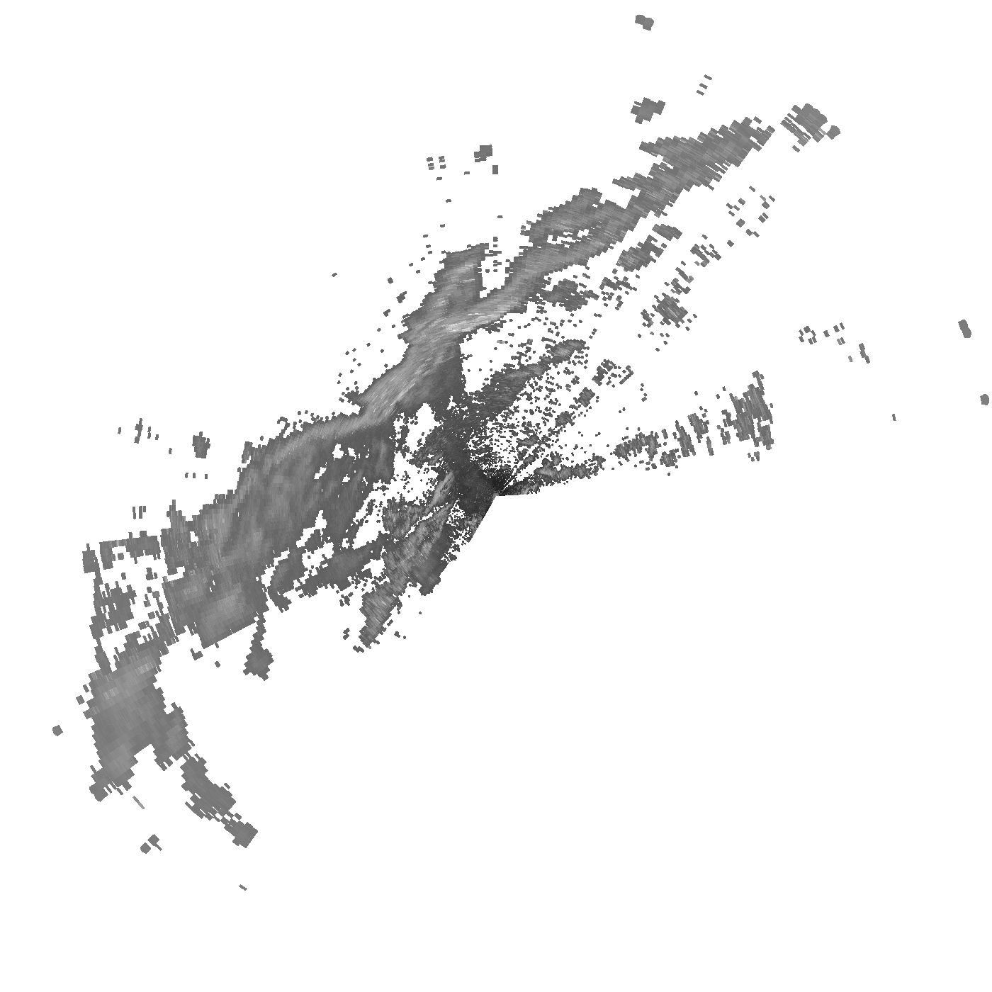
Translate exported GeoTiff to grayscale PNG

!gdal_translate -of PNG -ot Byte -scale -30. 60. 0 255 gridded_DBZH_20191021_082409.tif grayscale.png

Input file size is 1400, 1400
Warning 1: for band 1, nodata value has been clamped to 0, the original value being out of range.
0

...10...20...30...40...50...60...70...80...90...100 - done.

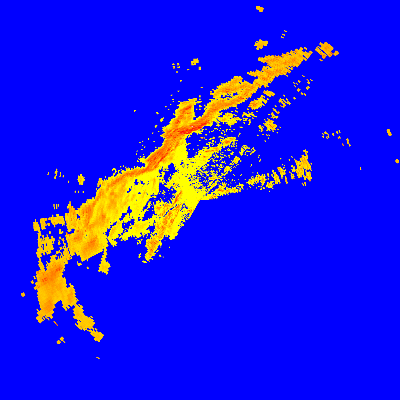
Apply colortable to PNG

with open("colors.txt", "w") as f:
    f.write("0 blue\n")
    f.write("50 yellow\n")
    f.write("100 yellow\n")
    f.write("150 orange\n")
    f.write("200 red\n")
    f.write("250 white\n")

Display exported PNG’s

!gdaldem color-relief grayscale.png colors.txt paletted.png

0...

10...20...30...40...50

...60...70...80...90...100 - done.

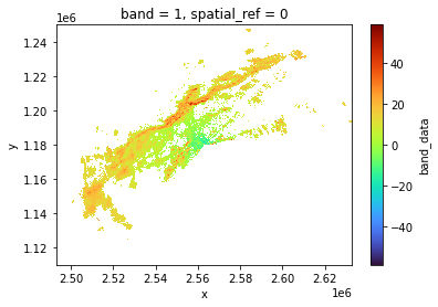
Import with Xarray, rasterio backend

with xr.open_dataset("gridded_DBZH_20191021_082409.tif", engine="rasterio") as ds_grd:
    display(ds_grd)
    ds_grd.band_data.plot(cmap="turbo")

/srv/conda/envs/notebook/lib/python3.9/site-packages/pyproj/crs/_cf1x8.py:511: UserWarning: angle from rectified to skew grid parameter lost in conversion to CF
  warnings.warn(

<xarray.Dataset>
Dimensions:      (band: 1, x: 1400, y: 1400)
Coordinates:
  * band         (band) int64 1
  * x            (x) float64 2.493e+06 2.493e+06 ... 2.633e+06 2.633e+06
  * y            (y) float64 1.25e+06 1.25e+06 1.25e+06 ... 1.11e+06 1.11e+06
    spatial_ref  int64 0
Data variables:
    band_data    (band, y, x) float32 ...

xarray.Dataset

• Dimensions:
  • band: 1
  • x: 1400
  • y: 1400
• Coordinates: (4)
  • band
    (band)
    int64
    1

    array([1])

  • x
    (x)
    float64
    2.493e+06 2.493e+06 ... 2.633e+06

    array([2493011., 2493111., 2493211., ..., 2632711., 2632811., 2632911.])

  • y
    (y)
    float64
    1.25e+06 1.25e+06 ... 1.11e+06

    array([1249920.625, 1249820.5  , 1249720.375, ..., 1110046.   , 1109945.875,
           1109845.75 ])

  • spatial_ref
    ()
    int64
    ...

    crs_wkt :

    PROJCS["CH1903+ / LV95",GEOGCS["CH1903+",DATUM["CH1903+",SPHEROID["Bessel 1841",6377397.155,299.1528128,AUTHORITY["EPSG","7004"]],AUTHORITY["EPSG","6150"]],PRIMEM["Greenwich",0,AUTHORITY["EPSG","8901"]],UNIT["degree",0.0174532925199433,AUTHORITY["EPSG","9122"]],AUTHORITY["EPSG","4150"]],PROJECTION["Hotine_Oblique_Mercator_Azimuth_Center"],PARAMETER["latitude_of_center",46.9524055555556],PARAMETER["longitude_of_center",7.43958333333333],PARAMETER["azimuth",90],PARAMETER["rectified_grid_angle",90],PARAMETER["scale_factor",1],PARAMETER["false_easting",2600000],PARAMETER["false_northing",1200000],UNIT["metre",1,AUTHORITY["EPSG","9001"]],AXIS["Easting",EAST],AXIS["Northing",NORTH],AUTHORITY["EPSG","2056"]]

    semi_major_axis :

    6377397.155

    semi_minor_axis :

    6356078.962818189

    inverse_flattening :

    299.1528128

    reference_ellipsoid_name :

    Bessel 1841

    longitude_of_prime_meridian :

    0.0

    prime_meridian_name :

    Greenwich

    geographic_crs_name :

    CH1903+

    horizontal_datum_name :

    CH1903+

    projected_crs_name :

    CH1903+ / LV95

    grid_mapping_name :

    oblique_mercator

    latitude_of_projection_origin :

    46.9524055555556

    longitude_of_projection_origin :

    7.43958333333333

    azimuth_of_central_line :

    90.0

    scale_factor_at_projection_origin :

    1.0

    false_easting :

    2600000.0

    false_northing :

    1200000.0

    spatial_ref :

    PROJCS["CH1903+ / LV95",GEOGCS["CH1903+",DATUM["CH1903+",SPHEROID["Bessel 1841",6377397.155,299.1528128,AUTHORITY["EPSG","7004"]],AUTHORITY["EPSG","6150"]],PRIMEM["Greenwich",0,AUTHORITY["EPSG","8901"]],UNIT["degree",0.0174532925199433,AUTHORITY["EPSG","9122"]],AUTHORITY["EPSG","4150"]],PROJECTION["Hotine_Oblique_Mercator_Azimuth_Center"],PARAMETER["latitude_of_center",46.9524055555556],PARAMETER["longitude_of_center",7.43958333333333],PARAMETER["azimuth",90],PARAMETER["rectified_grid_angle",90],PARAMETER["scale_factor",1],PARAMETER["false_easting",2600000],PARAMETER["false_northing",1200000],UNIT["metre",1,AUTHORITY["EPSG","9001"]],AXIS["Easting",EAST],AXIS["Northing",NORTH],AUTHORITY["EPSG","2056"]]

    GeoTransform :

    2492961.0 100.0 0.0 1249970.6875 0.0 -100.125

    array(0)

• Data variables: (1)
  • band_data
    (band, y, x)
    float32
    ...

    [1960000 values with dtype=float32]

• Attributes: (0)

---

Summary

We’ve just learned how to use \(\omega radlib\)’s xarray backends to make radar volume data available as xarray Datasets and DataArrays. Accessing, plotting and exporting data has been shown.

What’s next?

In the next notebook we dive into data quality processing.

Resources and references

• xarray

• dask

• matplotlib

• matplotlib axisartist

• cartopy

• gdal

• wradlib xarray backends

• rioxarray

• wradlib scan strategy

• Leonardo - Rainbow5

• OPERA ODIM_H5

• WMO JET-OWR

previous

An Overview of wradlib

next

wradlib data quality